 Gennaro Senatore
 Arka P. Reksowardojo
94% of researchers rate our articles as excellent or good
Learn more about the work of our research integrity team to safeguard the quality of each article we publish.
Find out more
ORIGINAL RESEARCH article
Front. Built Environ. , 22 July 2020
Sec. Computational Methods in Structural Engineering
Volume 6 - 2020 | https://doi.org/10.3389/fbuil.2020.00105
This article is part of the Research Topic Design and Control of Adaptive Civil Structures View all 13 articles
This work presents force and shape control strategies for adaptive structures subjected to quasi-static loading. The adaptive structures are designed using an integrated structure-control optimization method developed in previous work, which produces minimum “whole-life energy” configurations through element sizing and actuator placement optimization. The whole-life energy consists of an embodied part in the material and an operational part for structural adaptation during service. Depending on the layout, actuators are placed in series with the structural elements (internal) and/or at the supports (external). The effect of actuation is to modify the element forces and node positions through length changes of the internal actuators and/or displacements of the active supports. Through active control, the stress is homogenized and the displacements are kept within required limits so that the design is not governed by peak demands. Actuation has been modeled as a controlled non-elastic strain distribution, here referred to as eigenstrain. Any eigenstrain can be decomposed into two parts: an impotent eigenstrain only causes a change of geometry without altering element forces while a nilpotent eigenstrain modify element forces without causing displacements. Four control strategies are formulated: (C1) force and shape control to obtain prescribed changes of forces and node positions; (C2) shape control through impotent eigenstrain when only displacement compensation is required without affecting the forces; (C3) force control through nilpotent eigenstrain when displacement compensation is not required; and (C4) force and shape control through operational energy minimization. Closed-form solutions to decouple force and shape control through nilpotent and impotent eigenstrain are given. Simulations on a slender high-rise structure and an arch bridge are carried out to benchmark accuracy and energy requirements for each control strategy and for different actuator configurations that include active elements, active supports and a combination of both.
The construction sector is an important field of action in the on-going global effort to reduce anthropogenic greenhouse gas emissions (GHG) that aims to mitigate the potential consequence of climate crisis (I. E. Agency, 2018). Efforts to reduce building GHG emissions have focused mainly on operational emissions such as those that arise from heating/cooling, ventilation, lighting etc. However, a significant share of buildings and structures GHG life cycle emissions is embodied because it arises from the manufacturing of components, construction, transport and demolition (Bekker, 1982). Recent studies have highlighted that the average embodied share of life cycle GHG emissions is 45–50% for energy-efficient buildings and that considering a service life of 50 years, the contribution of embodied GHG emissions can reach and surpass a ratio of 1:1 (embodied:operational) (Röck et al., 2020). Load-bearing systems have an important share of the environmental impact embodied in the built environment due to the large amount of material required for their construction and energy-intensive fabrication processes (Cole and Kernan, 1996; Kaethner and Burridge, 2012). According to the International Energy Agency (IEA), the embodied carbon (EC) of building structures, substructures and enclosures is responsible for 28% of global building sector emissions (I. E. Agency, 2018). Rapid growth population in conjunction with current and future energy depletion and material scarcity (I. E. Agency, 2017), call for new and radical solutions to reduce structures material usage and environmental impact. Despite this, best practice in structural design has led to significant oversizing because the structure is designed to withstand worst-case loads with long return periods such as high winds, earthquakes, heavy snow and large crowds. Since load-bearing structures are typically subjected to loads that are significantly lower than the design loads, it means that most structures are overdesigned for the majority of their service life.
Active structural control through sensing and actuation has been investigated as a strategy to meet safety and serviceability requirements under strong loading events such as high winds, earthquakes and unusual crowds (Soong, 1988; Casciati et al., 2012). Adaptive structures can control forces and deflections to stay within required limits such that the effect of external loading is reduced instead of relying only on passive load-bearing resistance. Several systems have been studied to control the structural response including building frames equipped with active bracings/columns (Reinhorn et al., 1993; Wagner et al., 2018; Weidner et al., 2018) and variable stiffness joints (Wang et al., 2020) as well as bridges equipped with active cable-tendons (Rodellar et al., 2002; Xu et al., 2003). Through integrated structure-control optimization (Smith et al., 1991; Begg and Liu, 2000; Soong and Cimellaro, 2009; Frohlich et al., 2019) civil structures can be designed to adapt (e.g., react positively) to rare loading events of high intensity in order to operate closer to required limits, which results in a better material utilization compared to equivalent weight-optimized passive structures (Teuffel, 2004; Sobek, 2016; Böhm et al., 2019). Material savings, however, are only possible at a cost of energy that is required to operate the adaptive system.
A new integrated structure-control optimization method has been formulated by Senatore et al. (2019), which produces minimum “whole-life” energy structures. The whole-life energy consists of the energy embodied in the material for material extraction, fabrication and construction as well as the operational energy for control. The whole-life energy is a new design criterion that allows to obtain adaptive structural systems with a significantly reduced material mass and which are minimum energy solutions thus reducing environmental impacts with respect to conventional passive structures. Extensive numerical and experimental studies (Senatore et al., 2018a,c) have demonstrated that adaptive structures designed through the method given in Senatore et al. (2019), have significantly improved performances including reduced material mass, increased slenderness and increased stiffness as deflections are controlled within tight limits. In parallel, minimum energy adaptive structures have a lower environmental impact as the total energy can be reduced by up to 70% for slender configurations with respect to equivalent weight-optimized passive structures (Senatore et al., 2018b). Structural adaptation is particularly beneficial for stiffness governed design problems where it is challenging to reduce deflections within required limits for passive load-bearing systems. Instead, a well-designed adaptive structure can compensate for deflections actively at the cost of a small amount of operational energy. High-rise structures, long-span bridges and self-supporting roof systems are generally stiffness governed and therefore they are could greatly benefit from adaptive design strategies. Structural adaptation through geometric non-linear control has been further investigated in Reksowardojo et al. (2019, 2020a). Numerical and experimental studies have shown that when the structure is designed to be controlled into shape configurations that are optimal to counteract the effect of the external load, the stress can be effectively homogenized and minimized under different loading conditions. This leads to significant embodied energy savings with respect to adaptive structures limited to small shape changes as well as to weight-optimized passive structures.
The effect of actuation can be thought of as a non-elastic deformation that is similar to the strain caused by a lack of fit, thermal loading, plastic deformation or creep. This approach was taken in Ramesh and Utku (1991) and Lu et al. (1992) for force and geometry control as well as to formulate actuator placement optimization procedures. This type of non-elastic deformation has been referred to as eigenstrain in Mura (1991) and Irschik and Ziegler (2001). Nyashin et al. (2005) have shown that an eigenstrain can be decomposed into two main types: an impotent eigenstrain causes displacements without producing a stress change while a nilpotent eigenstrain changes the stress without causing displacements. This decomposition is of particular relevance in the context of active structural control because through inducing an impotent or a nilpotent eigenstrain, it is possible to control independently the external geometry and the forces, respectively.
The formulation of four control strategies in given in this paper: (C1) force and shape control to obtain prescribed changes of forces and node positions; (C2) shape control through impotent eigenstrain when only displacement compensation is required; (C3) force control through nilpotent eigenstrain when displacement compensation is not required and (C4) force and shape control through operational energy minimization. This work extends the integrated structure-control optimization method given in Senatore et al. (2019) with the formulation of control strategies C2, C3, and C4.
Depending on the actuator layout, actuators can be placed in series with the structural elements (internal actuator) and/or at the supports (external actuator). With a few exceptions such as in Neuhaeuser et al. (2013), force and shape control through active supports has received little attention. In Senatore et al. (2019) it was shown that the length change of a linear actuator integrated in a reticular structure, can be conveniently modeled through an eigenstrain assignment which becomes part of the external load. This work extends the force and shape control formulation given in Senatore et al. (2019) to include the action (controlled displacements) of active supports.
This paper is arranged in six sections. Section Synthesis of Minimum Energy Adaptive Structures gives a summary of the design method adopted in this work. Section Structural Adaptation Process defines the structural adaptation process and it outlines the main formulation adopted in this work for structural analysis and control. Section Control Strategies gives the formulation of control strategies C1, C2, C3, and C4. In Section Case Studies, strategies C1, C2, C3, and C4 are applied to the control of a slender high-rise structure and an arch-truss bridge. Section Discussion and Conclusions conclude the paper.
This work builds on the design method for adaptive structures given in Senatore et al. (2019). This method synthesizes adaptive structures through minimization of the whole-life energy (or total energy). The ability to actively counteract the effect of loading generally results in large savings of material and thus embodied energy. To minimize the consumption of operational energy for control, the structure is designed to rely on passive load-bearing capacity under normal loading conditions while adaptation is employed under strong loading events that occur rarely. This way, the embodied energy in the material is reduced at a small cost of operational energy. The formulation has been implemented for reticular structures with the assumption of small strains and small displacements. Note that it is assumed the dynamic response is not controlled through the active system. For the same reason, seismic design criteria are not included. Also, since adaptation is only necessary against strong but rare loads, it is assumed that fatigue is not a critical limit state.
The design variables are the element cross-section areas, the element forces, the actuator placement and the control commands. The objective is to minimize embodied and operational energy subject to ultimate and serviceability limit states under a randomly varying external load. Optimization is carried out through a nested scheme. Embodied and operational energy optimization are coordinated through two auxiliary variables: a design variable denoted as Material Utilization (MUT) factor which can be thought of as demand over capacity ratio defined for the structure as a whole; a state variable denoted as Load Activation Threshold (LAT) which is the lowest intensity loading event that causes a violation of a limit state. In the outer process, the MUT is varied in the range of 0% < MUT ≤ 100% to obtain the minimum energy configuration. Figure 1A shows a notional relationship of the whole-life energy as a function of the MUT. A small MUT produces a very light-weight structure which has a small embodied energy but it might require large control energy to satisfy stress and displacements limits during service (i.e., low level of LAT). Vice versa, a high MUT results into a stiffer structure which embodies larger energy in the material but it requires smaller control energy (i.e., high level of LAT).
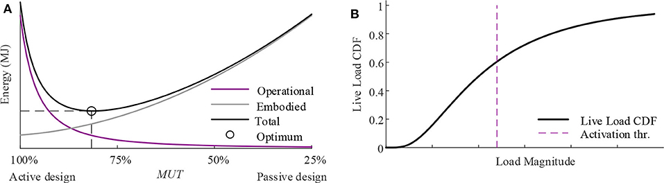
Figure 1. (A) Embodied, operational, and whole-life energy as a function of the Material Utilization Factor (MUT); (B) live load Cumulative Distribution Function (CDF) (Senatore et al., 2019).
For each MUT three steps are carried out: (1) embodied energy minimization, (2) actuator placement optimization, and (3) operational energy computation.
The embodied energy is minimized through optimization of the element cross-section sizing and the internal load path (i.e., element forces). The embodied energy is computed for each element by scaling its mass with a material energy intensity factor which is the energy per unit mass for extraction and manufacturing taken from the Inventory of Carbon and Energy (ICE) (Hammond and Jones, 2008). For clarity, when all the structural elements are made of a single material, the embodied energy is equal to the mass scaled by a single factor.
This process can be thought of as a mapping between external loads, element forces and nodal displacements:
the index j refers to the jth load case and np is the total number of load cases. The superscript t stands for target to denote the optimal internal load path. The outputs of this process are the cross-section areas and target forces ftunder each load case.
Embodied energy optimization is carried out subject to equilibrium and ultimate limit state (ULS) constraints which include admissible stress and element buckling. However, geometric compatibility and deflection limits i.e., serviceability limit state (SLS) are not part of the optimization constraints. This means that when the load is applied and geometric compatibility is considered, the forces f will be, in general, different to the target ones ft obtained through χ and the node displacements d might not be within the required serviceability limits dt. The computation of dt requires selecting the controlled nodes (or controlled degrees of freedoms, denoted with cd) which is an input to the optimization process. The choice of cd depends on the type of structure as well as serviceability criteria. When the load causes a violation of an ultimate and/or a serviceability limit state, the forces and node positions will be controlled through actuation.
The actuator layout comprises linear actuators which are assumed to be installed in series with the structure elements as shown by the illustrations in Table 1. The action of a linear actuator is to expand or retract, which is simulated through a non-elastic change of length Δl of the element onto which is fitted. The effect of the actuator length changes is to cause a change of forces Δfc and node positions Δdc (i.e., a change of shape). When the load causes a violation of an ultimate and/or a serviceability limit state, appropriate actuator commands Δl are computed to cause a change of forces Δft = ft − f from a compatible state f to the target state ft (obtained through χ) and a change of shape Δdt = dt − d from the deformed shape d to the target one dt required by SLS.
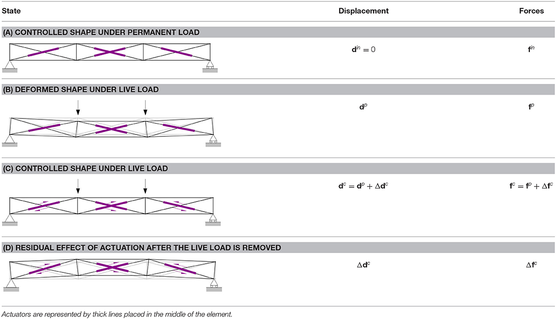
Table 1. Structural adaptation process.
The actuator placement optimization is a combinatorial problem which involves placing a certain number of linear actuators within a set of available sites (the structural elements or the supports). In order to improve computational efficiency, this binary problem has been relaxed into a continuous form through sensitivity analysis (Senatore et al., 2019). The actuators are placed through ranking by employing a control efficacy measure which evaluates the contribution of each actuator toward the attainment of the target change of forces Δft and node positions Δdt. The objective is to obtain an actuator layout so that the change of forces Δfc and node positions Δdc caused by Δl are as close as possible to the required Δft and Δdt, respectively:
where 𝔸ℂ𝕋 ∈ ℤnact; 𝔸ℂ𝕋 ⊆ {1, …, ne} is the set which contains the element indices that denote the actuator locations. When the actuator placement is known, suitable actuator commands Δl are obtained to control the structure through the target change of forces Δft and node positions Δdt. This is an inverse problem which has been solved through constrained optimization as described in section Control to Target Forces and Shapes (C1).
Once the actuator layout is known, it is possible to compute the actuation system embodied energy which is added to the structure embodied energy obtained from step 1. The same applies to the mass of the adaptive solution which is the sum of the structure mass and the actuation system mass. Generally, it is reasonable to assume that the actuator embodied energy (and thus its mass) increases as the actuator force capacity increases. In Senatore et al. (2019), it has been assumed that an actuator is entirely made of steel with an energy intensity of 35 MJ/kg (Hammond and Jones, 2008) and its mass is a proportional to the required force capacity (i.e., the maximum force required through control) with a constant of 0.1 kg/kN (e.g., an actuator with a push/pull load of 10,000 kN has a mass of 1,000 kg) (ENERPAC, 2016).
Embodied energy optimization and actuator layout optimization are interrelated because the actuation system is an integral part of the structure. The layout of the structure (produced by process χ in Step 1) is obtained with the assumption that serviceability requirements are met through active control. Conversely, the optimal actuator placement that is determined through process ϑ depends on the layout of the structure produced by process χ. The actuator efficacy to control internal forces and displacements depends on its location in the structure as well as the position of the control nodes. The actuator optimal layout changes as the MUT is varied during energy optimization because the material distribution changes and therefore also the required force control and displacement compensation change.
The structure is subjected to a permanent (self-weight + dead load) and a randomly fluctuating live load. For simplicity, all loads that are not permanent are considered live loads including events such as high winds, unusual crowds etc. The probability distribution of the live load is modeled with a log-normal function which is suitable to model a generic random occurrence. Figure 1B shows the plot of a generic log-normal cumulative distribution where the load activation threshold LAT is indicated by a dashed line. The LAT is the lowest level of the load probability distribution that causes a state of stress and/or displacement to violate a limit state. The design load is set as the characteristic value which corresponds to the 95th percentile of the associated normal distribution. Since the operational energy is computed during service, the characteristic value is the design load without load factors (i.e., SLS load case). The load probability distribution is discretized into nd bins, the load corresponding to the kth bin (i.e., occurrence) is denoted as pjk. The discretized probability density is scaled by the expected service life of the structure which is usually set to 50 years. The duration of each loading event Δtjk is obtained through scaling the expected service life of the structure with the probability of the kth occurrence for the jth load case. The total operational energy is the sum of the energy required for force and displacement compensation for all the load occurrences above that corresponding to the LAT.
Steps 1 to 3 are repeated for each MUT to obtain the configuration of minimum energy. Although embodied and operational energy optimization are not carried out simultaneously (nested approach), it has been proven by Wang and Senatore (2020) that solutions produced by this method are only marginally different in energy terms to those produced by an All-in-One implementation of the same method through Mixed-Integer Non-linear Programming.
Table 1 gives an illustration of the four main states of the adaptation process considered in this work. The structure is controlled to move from the state (a) to state (d) for each load case. There are two phases of adaptation: (1) in the 1st phase (b–c), the structure is controlled to counteract the effect of the live load, (2) in the 2nd phase (d–a), the structure is controlled to eliminate the residual effect caused by actuation in the first phase, after the live load is removed.
The formulation presented in this study is implemented with the assumption of small strains and small displacements, and thus superposition applies. fin denote the forces when the structure is subjected only to permanent load which is assumed to be counteracted through actuation before the live load is applied. This can be thought of as a pre-cambering so that the structure undeformed (the displacements are reduced to zero, i.e., din = 0) when the live load is applied. fp and dp denote forces and displacements caused by the external load p. Δfc and Δdc are the change of forces and displacements caused by the actuator commands Δl. The forces and displacements at the start (b) and end (c) of the 1st phase are fp, dp and fc, dc, respectively. The forces and displacements at the start (d) and end (a) of the 2nd phase are fin + Δfc, din + Δdcand fin, din, respectively.
The analysis and control strategies implemented in this work use a force method formulation based on singular value decomposition of the equilibrium conditions in matrix form (Pellegrino and Calladine, 1986; Pellegrino, 1993), which is here referred to as SVD-FM. In previous own work (Reksowardojo and Senatore, 2020), it was proven that the SVD-FM is equivalent to the Integrated Force Method (IFM) (Patnaik, 1973) that was employed in Senatore et al. (2019) for design and control of adaptive structures. Both SVD-FM and IFM offer an effective way to predict the static response of a reticular structure subjected to external load and actuator actions. With these methods, actuation can be modeled as the effect of an imposed strain distribution i.e., eigenstrain, which is assigned directly as part of the external load. Although the IFM has a simpler and more intuitive formulation, the SVD-FM offers a way to derive closed-form solutions for control strategies C2 and C3 (impotent and nilpotent eigenstrain) which is the main reason it has been adopted in this work.
Given a pin-jointed structure made of ne elements, nn nodes in dim dimensions and thus having nd = dim · nn degrees of freedom, force-equilibrium conditions at nodes are:
where p ∈ ℝnd×1 is the external load vector. A ∈ ℝnd×(ne+nsd) is an extended equilibrium matrix which concatenates Ael ∈ ℝnd×neand Asup ∈ ℝnd×nsd:
Ael is the familiar equilibrium matrix which contains the element direction cosines. Details regarding the computation of Ael can be found in Pellegrino and Calladine (1986) and Achtziger (2007). Asup is a matrix that contains the support reaction direction cosines for nsdconstrained degrees of freedom. The supports are effectively thought of as infinitely rigid elements which constrain the rigid body motion of the structure. When the support reaction directions coincide with the global axes, as in most cases, Asup is a matrix containing zeros and ones.
The vector of forces f ∈ ℝ(ne+nsd) ×1 is the concatenation of the internal element forces fel ∈ ℝne×1 with the support reactions fsup ∈ ℝnsd×1:
Depending on the actuator layout, actuators can be placed in series with the structural elements (internal actuator) and/or at the supports (external actuator). An internal actuator is a linear actuator that can either extend or reduce the length of the element onto which it is fitted. An external actuator instead moves the position of a support which can be thought of as an induced differential settlement. The vector of actuator commands Δl ∈ ℝ(ne+nsd) ×1 is defined as the concatenation of the internal actuator length changes Δlel ∈ ℝne×1 with the support displacements caused by external actuators (or active supports) Δdsup ∈ ℝnsd×1:
Note that, once the actuator placement is determined, the actuator command vector Δl reduces its dimension to ℝ(nact) ×1 by including only the entries that correspond to the selected internal or external actuators.
Denote with r the rank of the equilibrium matrix A, then the number of self-stress states is s = (ne + nsd) − r and the number of mechanism modes is m = nd – r (including rigid body motion). Depending on the structural topology and the number of supports, static indeterminacy is caused by internal sint and/or external sext self-stress states such that s = sint + sext.
The singular value decomposition of A gives the following:
, and are the left singular vectors, right singular vectors and singular values of A, respectively. The term is the basis of the load components that are in equilibrium with the forces lying in the space spanned by which is the basis of the row space of A. The term is the basis of the null space of A. The columns of Ws are s linear independent states of self-stress. The term is the basis of the left null space of the equilibrium matrix . The columns of Um are m independent nodal displacement modes which do not cause first-order deformation of the elements i.e., the inextensional mechanism basis. If the external load has components that lie in the space spanned by Um, it will excite one or more mechanisms and therefore the structure will not be able to take the load in its original configuration. If only first-order infinitesimal mechanisms exist, appropriate prestress might be applied to stabilize the structure (Pellegrino, 1990). For kinematically determinate structures, Um does not exist. This work only considers structures with static indeterminacy but not kinematic indeterminacy. For the full static and kinematic interpretation of the terms obtained from the SVD of the equilibrium matrix, the reader is referred to Pellegrino (1993).
Recalling the equilibrium conditions in Equation 3, there is an infinite number of non-trivial solutions for the homogeneous system Af = 0 which are linear combinations of the self-stress vectors:
The particular solution instead is:
where A+ is the Moore-Penrose pseudoinverse of A, which can be computed as:
The general solution is the sum of the particular and homogeneous solutions:
where the operator ⊕ indicates a vector space addition. The linear coefficient vector μ is:
which is obtained by substituting into the compatibility conditions:
and then solving for μ. The term G ∈ ℝ(ne+nsd)×(ne+nsd) is the member flexibility matrix. For reticular structures G is a diagonal matrix with entries li/(Eiαi), where li, Ei and αi are the length, Young's modulus and cross-section area of the ith element of the structure ∀i ≤ ne. The entries of G are zeros for the supports i.e., ∀i > ne, since supports are assumed to be infinitely stiff. The s compatibility conditions in Equation 13 can be derived from virtual work or alternatively as shown in Pellegrino (1993) from the orthogonality between the compatible strains ε = Gf + Δl and the basis of incompatible strains Ws (Ws can be interpreted as both the self-stress and incompatible strain basis). Note that since the equilibrium matrix includes the support reaction direction cosines (Equation 4), each column of Ws includes support reactions that are in equilibrium with the self-stress state. The term ε includes the elastic strain Gf caused by the internal forces as well as the effect of a non-elastic strain Δl, i.e., eigenstrain, which could be produced by a lack of fit or thermal loading or, following Senatore et al. (2019), by the length change of internal actuators and/or external actuators (i.e., displacements of the active supports). Through Equation 11, the forces f caused by the combined effect (fp + Δfc) of the external load p and actuator commands Δl are computed through a single statement. When the actuator commands are included in Equation 11, the forces are denoted as fc i.e., controlled forces and otherwise as fp.
Considering only kinematically determinate structures and recalling the compatibility conditions ATd = Gf + ΔI, the node displacements d ∈ ℝndcaused by the combined effect (dp + Δdc) of the external load p and the actuator commands Δl are obtained as:
For kinematically determinate structure AT is a full column rank matrix and hence its pseudoinverse is unique. When the actuator commands Δl are included in Equation 14, the displacements are denoted as dc i.e., controlled displacements (or shape) and otherwise as dp.
Assuming small deformations, control through the actuator commands Δl (internal + external) causes a change of forces Δfc and shape Δdc, which can be expressed in matrix-vector product form as:
where and are defined as the force and shape influence matrix, respectively. Note that in Equations 15 and 16, ΔlAll ∈ ℝ(ne+nsd) ×1 contains control commands for all the elements and supports as if they were all active.
The force and shape influence matrices can be obtained by collating column-wise the effect of a unitary length change of each element and a unitary displacement of each support in turn on forces (Equation 11) and node positions (Equation 14) without applying any external load P (Senatore et al., 2019). However, from Equations 11 and 14, Sf and Sd can be also computed directly (as also shown in Yuan et al., 2016; Reksowardojo and Senatore, 2020):
where I denotes an identity matrix of dimensions (ne + nsd) × (ne + nsd).
The four strategies described in this section solve a common problem, which is the computation of suitable control commands given an actuator layout and a control objective. As anticipated in Step 2: Actuator Placement Optimization, following the method given in Senatore et al. (2019) control commands are computed to cause a simultaneous change of forces and node positions (C1) at the occurrence of a load above the activation threshold (LAT). However, in other cases, it might not be necessary to obtain a prescribed change of forces and node positions simultaneously. For example, it might be desirable to control only the node positions to satisfy deflection limits without affecting the forces if they are already within required limits (stress and stability). This can be achieved by applying an impotent eigenstrain through actuation (C2). Conversely, when it is only necessary to control the forces, for example, to reduce the stress under critical loading conditions but displacement compensation is not required, a possible strategy is to apply a nilpotent eigenstrain through actuation (C3). Finally, when the energy consumption of the actuation system is of primary concern, an alternative strategy is to obtain control commands through minimization of the work done by the actuators (C4) to minimize the operational energy during service.
Following the method given in Senatore et al. (2019) when the load causes a violation of an ultimate and/or a serviceability limit state, appropriate actuator commands Δl are computed to cause a change of forces Δft from a compatible state to the target state (obtained through χ) and a change of shape Δdt from the deformed shape to the target one required by SLS. For control strategy C1 (as well as C2 and C3), it is useful to distinguish between target change of forces Δft and shape Δdt and controlled change of forces Δfc and shape Δdc. The target state is given as an input. The objective is to obtain control commands Δl whose effect is to cause a Δfc and Δdc which are as close as possible to Δftand Δdt. This objective can be fulfilled with an accuracy that depends on the actuator layout.
The combined number of internal and external actuators is denoted as nact i.e., nact = nact,int + nact,ext. The number of controlled degrees of freedom is denoted as ncd. Recalling Equations 17 and 18, the force and shape influence matrices are computed assuming that all elements and supports are active. However, in practice only some of the elements and supports are equipped with actuators nact ≤ ne + nsd and it is required to control only some of the degrees of freedoms ncd ≤ nd. Assume an actuator layout with nactactuators and ncdcontrolled degree of freedom. The force influence matrix is reduced to which contains only the columns corresponding to the active elements and supports. Similarly, the shape influence matrix is reduced to which contains only the rows corresponding to controlled degrees of freedom and the columns corresponding to active elements and supports. The target shape change is also reduced to Δdt* ∈ ℝncd which contains only the entries corresponding to the controlled degrees of freedom. The same applies to the controlled shape change which is reduced to Δdc* ∈ ℝncd.
Since it is generally desirable to control structures with a simple (i.e., low number of actuators) actuation system, and are usually rectangular matrices with significantly more rows than columns (i.e., an over determinate linear system). A general formulation to compute actuator commands Δl to cause Δft and Δdt is through a constrained least square optimization:
The actuator commands Δl produced as the solution to this problem cause the required change of target force Δft and shape Δdt*. Generally, the rank of the reduced force and shape influence matrices and are equal to the degree of static indeterminacy s and the number of controlled degrees of freedom ncd, respectively. When this is the case, depending on a well-chosen actuator placement, if the number of actuators is set to nact = s + ncd the problem stated in Equations 19 and 20 admits a unique solution with low residuals (Δfc = Δft; Δdc* ≈ Δdt*). However, in practice it is generally preferable to reduce the number of actuators as much as possible. If the number of actuators is kept in the range s < nact ≤ s + ncd, generally force control can be carried out accurately (the equality constraint in Equation 20 is satisfied) but shape control will be approximate (Δfc = Δft; Δdc* ~ Δdt*). Depending on the choice of the controlled degrees of freedom and the actuator placement, there are cases in which or might be ill-conditioned. In these cases, adding more actuators might help to solve numerical issues.
In this work, the effect of actuation is modeled as a non-elastic deformation that is similar to the strain caused by thermal effect, plastic deformation or creep. This type of non-elastic deformation has been referred to as eigenstrain. Any eigenstrain can be uniquely decomposed into two distributions (Nyashin et al., 2005): impotent eigenstrain change the node positions without producing stress while nilpotent eigenstrain redistribute the stress without causing displacements. Impotent eigenstrain through actuation is useful when it is required to control the node positions without affecting the forces. Conversely, when it is only necessary to control the forces, a nilpotent eigenstrain could be applied through actuation.
An impotent eigenstrain is produced by actuator commands that cause a required change of node positions Δdt without changing the forces, therefore:
Equation 22 is a homogeneous linear equation system whose trivial solution is Δlall = 0. Assuming that all elements and supports are active, there is an infinite number of non-trivial solutions:
where Wr is the basis of the row space of the equilibrium matrix A which is defined in section Analysis and Control of Adaptive Structures. Recalling Equation 17 for the force influence matrix Sf, the product of with any linear combination of Wr vanishes since by definition the row space is orthogonal to the null space. Therefore, if the actuator command components lie in the space spanned by Wr, it will produce an impotent eigenstrain. Replacing Equation 23 in Equation 21 and then solving for β:
Therefore, Δlall to produce an impotent eigenstrain is:
Assuming small deformations, Equation 25 gives actuator commands Δlall which cause the required change of node positions Δdc = Δdt and no change of forces Δfc = 0. This means that the node positions change only through non-elastic deformations that do not cause any elastic deformation of the elements.
If only selected elements are actuators and only selected degrees of freedom are controlled, the non-trivial solutions of Equation 22 are actuator commands whose components lie in the null space of the reduced force influence matrix :
Replacing Equation 26 in Equation 21 and solving for Δl:
where is the basis of the null space of i.e., . Equation 27 gives actuator commandsΔl which cause a change of node positions Δdc* ~ Δdt* and no change of forces Δfc = 0. Δdc* caused by Δl is not exactly Δdt* because only some of the elements or supports are active, the degree of accuracy depends on the actuator placement and the number of actuators. Note that Equation 27 produces a non-zero Δl vector provided that the nullity of is not zero. Since is a rank deficient matrix of rank s (i.e., the degree of static indeterminacy), the nullity of is greater than zero only if the number of internal actuators is greater than sint i.e., nact,int > sint. Otherwise when nact,int ≤ sint, the columns of are linearly independent and therefore the nullity is zero i.e., the linear system admits only the trivial solution of Δl = 0. When external actuators (i.e., active supports) are employed, the requirement nact,int > sint does not apply. Instead, impotent eigenstrain can be caused by actuator commands computed through Equation 27 if the number of active supports is greater than sext i.e., nact,ext > sext. When internal and external actuators are employed in combination, Equation 27 can be used if sext < nact,ext ∪ sint < nact,int is true.
For the case when the nullity of is zero (nact,ext ≤ sext ∪ nact,int ≤ sint) and if a small change of forces is admissible, displacements can be controlled through an approximate impotent eigenstrain by solving the following constrained optimization problem:
The actuator commands Δl obtained from the solution of the problem stated in Equations 28 and 29 cause the required change of node positions Δdc* = Δdt* through a minimum change of forces Δfc ~ 0, which can be thought of as the effect of an approximate impotent eigenstrain. Similar to C1, if the number of actuators is set to nact = s + ncd the problem stated in Equations 28 and 29 admits a unique solution with low residuals (Δfc ≈ 0;Δdc* = Δdt*). However, note that a significant change of forces may occur when nact,int ≤ sint. Equations 28 and 29 may also be used in cases where Equation 27 yields Δl → ∞ because is ill-conditioned. Table 2 gives a summary of the different approaches to obtain control commands that cause an impotent eigenstrain. Control accuracy decreases as the number of actuators reduces from nact,int = ne or nact,ext = nsd (all elements or supports are active) to nact,int = sint or nact,ext = sext in which cases it is no longer possible to control the shape without also causing a change of forces.
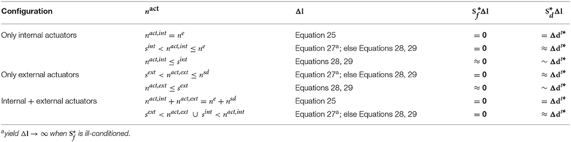
Table 2. Shape control through impotent eigenstrain.
A nilpotent eigenstrain is produced by actuator commands that cause a change of forces but no change of displacements:
Equation 31 has a trivial solution for Δlall = 0. Assuming that all elements and supports are active, there is an infinite number of non-trivial solutions:
Equation 32 can be derived by expanding Equation 31 through Equations 17 and 18 and replacing Δlall with GWsδ:
The underlined term is an identity matrix and therefore the right-hand term vanishes. This proves that any Δlall spanning GWs causes no change of node positions. Replacing Equation 32 into Equation 30 and then solving for δ:
Therefore, Δlall to produce a nilpotent eigenstrain is:
Assuming small deformations, Equation 35 gives actuator commands Δlall which cause the required change of forces Δfc = Δft and no change of shape Δdc* = 0. Note that force control through nilpotent eigenstrain can be performed with good accuracy only if the target force change is a linear combination of the s column vectors of Ws.
If only selected elements are actuators the non-trivial solutions of Equation 31 are actuator commands whose components lie in the null space of the reduced shape influence matrix :
Replacing Equation 36 in Equation 30 and solving for Δl:
where is the basis of the null space of i.e., . Equation 37 gives actuator commands Δl that cause a change of forces Δfc ~ Δft and no change of shape Δdc* = 0. Δfc caused by Δl is not exactly Δft because only some of the elements or supports are active, the degree of accuracy depends on the actuator placement. Note that Equation 37 produces a non-zero Δl vector provided that the nullity of is not zero. Referring to the rank-nullity theorem, since is a full row rank matrix, the nullity of is greater than zero only if the number of internal actuators is greater than the number of controlled degrees of freedom i.e., nact,int > ncd. Otherwise when nact,int ≤ ncd, becomes a full rank matrix which has a nullity of zero and thus the linear system can only admit the trivial solution Δl = 0. Note that it is not possible to obtain actuator commands that cause a nilpotent eigenstrain through Equation 37 when active supports are employed. This is because the effect of an active support is to move the node position and therefore by definition it cannot be employed to produce a nilpotent eigenstrain. In addition, in some configurations that include internal and external actuators, might be ill-conditioned. In this case, Equation 37 yields Δ l → ∞.
For the case when the nullity of is zero because nact,int ≤ ncd and when active supports are employed, if a small change of shape is admissible, forces can be controlled through an approximate nilpotent eigenstrain by solving the following constrained optimization problem:
The actuator commands Δl obtained from the solution of the problem stated in Equations 38 and 39 cause the required change of forces Δfc = Δft through a minimum change of node positions Δdc* ~ 0, which can be thought of as the effect of an approximate nilpotent eigenstrain. Similar to C1 and C2, if the number of actuators is set to nact = s+ncd the problem stated in Equations 38 and 39 admits a unique solution with low residuals (Δfc = Δft; Δdc* ≈ 0). However, note that a significant change of node positions may occur when nact,int < ncd. Equations 38 and 39 may also be used in cases where Equation 37 yields Δl → ∞ because is ill-conditioned.
Table 3 gives a summary of the different approaches to obtain control commands that cause a nilpotent eigenstrain. Control accuracy decreases as the number of actuators reduces from nact,int = ne (all elements are active) to nact,int = ncd in which case it is no longer possible to control the forces without also causing a change of node positions. It is generally not possible to compute control commands that cause a nilpotent eigenstrain through Equation 37 if active supports are employed. However, active supports can be used through Equations 38 and 39.
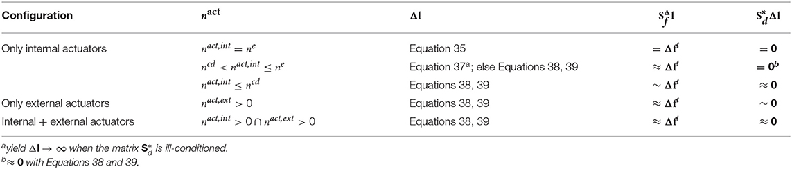
Table 3. Force control through nilpotent eigenstrain.
When operational energy consumptions are of primary concern, control commands Δl can be obtained through minimization of the work done by the actuators subject to stress and deflection limits. In this case, no target change of forces Δft and node positions Δdt are supplied as inputs. The objective is to obtain suitable control commands so that forces fc and displacements dc are controlled as required by ULS and SLS, respectively, using minimum energy. Assuming small deformations and a linear elastic force-displacement relationship, the actuator work is made of two parts:
where fp are the forces before control which are assumed constant during actuation and Δfc is the change of forces caused by the actuator commands Δl. The objective function is sign-dependent because an actuator does work only when the applied forces and the length (internal) or displacement (support) changes are of opposite signs. For example, work is done when an internal actuator is required to extend under compression or to contract under tension and an external actuator is required to move the support in the opposite direction of the force it receives from the structure (opposite in sign of the support reaction). Otherwise, theoretically there would be a release of energy but since this study does not consider energy harvesting solutions, it is assumed that no energy gain can be made.
The total operational energy during service is computed as:
and are the work done during the first (1) and second (2) phase of adaptation (see section Structural Adaptation Process), respectively, by the ith actuator, under the jth load case for the kth occurrence (i.e., bin) of the load probability distribution which, in this work, is assumed to be a log-normal distribution as defined in Step 3: Operational Energy Computation. Δtjk is the duration of the load occurrence which is obtained through scaling the expected life-span of the structure with the probability of the kth occurrence for the jth load case pjk. As discussed in Step 3: Operational Energy Computation, only load occurrences that are above the load activation threshold (LAT), which is denoted by k*, are accounted for. The actuator working frequency ω is assumed to be identical to the 1st natural frequency which is likely to dominate the response of the structure. The actuator mechanical efficiency η is set depending on the actuator specification. For more details regarding the computation of the operational energy, the reader is referred to Senatore et al. (2019).
Minimization of the operational energy is subject to stress and displacement constraints to satisfy ULS and SLS:
This formulation follows a Simultaneous Analysis and Design approach (Haftka, 1985) which was developed in previous own work (Wang and Senatore, 2020). The design variables vector xcomprises the actuator work as well as the control commands:
The actuator work is reformulated using two auxiliary variables:
subject to auxiliary constraints (Equations 49–54). The auxiliary variables , and constraints are introduced to handle the sign-dependency of the optimization objective in order to formulate it as a continuous function. Note that Equation 56 is satisfied only at convergence i.e., when reaches a minimum. The superscript (1) and (2) in the auxiliary constraints refer to the 1st and 2nd phase of the adaptation process (Section Structural Adaptation Process).
Similar to C1, C2, and C3, stress and displacement constraints in Equations 45–47 employ the force and shape and influence matrices to relate the actuator commands Δl to the controlled change of forces and node positions , respectively. The change of forces is obtained so that the controlled forces fc = fp + Δfc, where fp are the forces caused by the external load before control, are constrained by stress and stability limits (Equation 45 and 46). The change of node positions Δdc is obtained so that the controlled displacements dc = dp + Δdc, where dp are the displacements caused by the external load before control, are bounded by SLS limits (Equation 47). The actuator commands Δl are also constrained to stay within required limits which are specific to the selected actuation system (Equation 48).
The optimization problem stated in Equations 44 to 54 has been successfully solved for the case studies presented in this work using the Sequential Quadratic Programming (SQP) algorithm built-in Matlab. Note that since the problem is generally non-convex, the optimal solutions obtained through SQP are local minima. Since control commands obtained through C4 require minimum operational energy, this strategy will be used to benchmark the energy requirements of C1, C2, and C3.
The structure-control optimization method outlined in section Synthesis of Minimum Energy Adaptive Structures (Senatore et al., 2019) combined with the control strategies given in section Control Strategies has been applied to the design of a high-rise structure and an arch bridge. The main objective of the comparative study presented in this section is to benchmark the control strategies to evaluate energy requirements and control accuracy.
The four control strategy described in section Control Strategies are compared: (C1) force and shape control to obtain prescribed changes of forces and node positions, (C2) shape control through impotent eigenstrain, (C3) force control through nilpotent eigenstrain, and (C4) force and shape control through operational energy minimization. For all control strategies, three actuator configurations (AC) are considered: only internal actuators (AC1), only external actuators (AC2) and a combination of both (AC3). The control strategies and related actuator configurations are compared in terms of:
• Maximum controlled displacement max (|dp+Δdc − din|) to evaluate if the required SLS limit is met
• Control residuals with respect to target force and shape changes
• Maximum element force change max (|Δfc|)caused by actuation
• Maximum shape change max (|Δdc|)caused by actuation
• Maximum actuator force capacity max (|f|) ∀i ∈ 𝔸ℂ𝕋
• Maximum internal actuator length extensionmax (Δlel)and reduction min (Δlel)
• Maximum active support displacement max (Δdsup); min (Δdsup)
• Embodied and operational energy as well as mass and energy savings with respect to the passive solution
• Computation time to obtain control commands Δl.
Since actuators are assumed to be installed in series, they have to carry the full force in the corresponding element or support. For this reason, the maximum actuator force capacity is computed as the maximum force (in absolute value) that an actuator has to withstand over the entire adaptation process, namely the maximum among fin, fp, fc and fin + Δfc (see section Analysis and Control of Adaptive Structures). For simplicity of notation, this is indicated as max (|f|). With regard to the internal actuator length changes, a positive sign indicates an extension whereas a negative sign a length reduction. For external actuators, a positive sign indicates that the displacement is applied in the same direction of the support axis.
In both cases studies, the structures are made of circular hollow section elements. The minimum radius is set to 50 mm and 100 mm for the high-rise structure and the arch bridge configurations, respectively. To limit optimization complexity, the wall thickness is set to 10% of the external radius. The element material is structural steel with a Young's modulus of 210 GPA, a density of 7,850 kg/m3 and an energy intensity of 36.5 MJ/kg (Hammond and Jones, 2008). Following Senatore et al. (2019), it is assumed that the actuators are made of steel with an energy intensity factor of 36.5 MJ/kg and the actuator mass is linearly proportional to the required force capacity (i.e., maximum force required during control) with a coefficient of 0.1 kg/kN (e.g. an actuator with a push/pull load of 10,000 kN has a mass of 1,000 kg) (ENERPAC, 2016). Note that the mass of the adaptive configuration includes the mass of the actuation system layout. The same applies to the embodied energy. Similarly, the self-weight of the adaptive configuration comprises the weight of the structure and that of the actuation system.
The structure is subjected to a permanent load, which comprises self-weight (SW) and dead load (DL), as well as to a randomly fluctuating live load (LL) whose frequency of occurrence is modeled with a log-normal probability distribution (see section Step 3: Operational Energy Computation). The load combination cases considered in the case studies are summarized in Table 4.
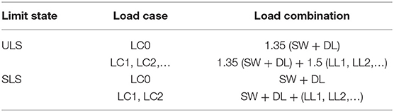
Table 4. Load combination cases.
The vertical cantilever truss considered in this study can be thought of as the primary structure of a multi-story building reduced to two dimensions. The geometry of the structure is illustrated in Figure 2A which shows dimensions, support and loading conditions. The horizontal displacements of all free nodes are set as controlled degrees of freedom for a total of ncd = 16. The controlled nodes are indicated by circles. The serviceability limit is set to H / 500 = 200 mm, where H = 100 m is the height of the structure. The degree of static indeterminacy (s) is sint = 7 internally and sext = 1 externally.
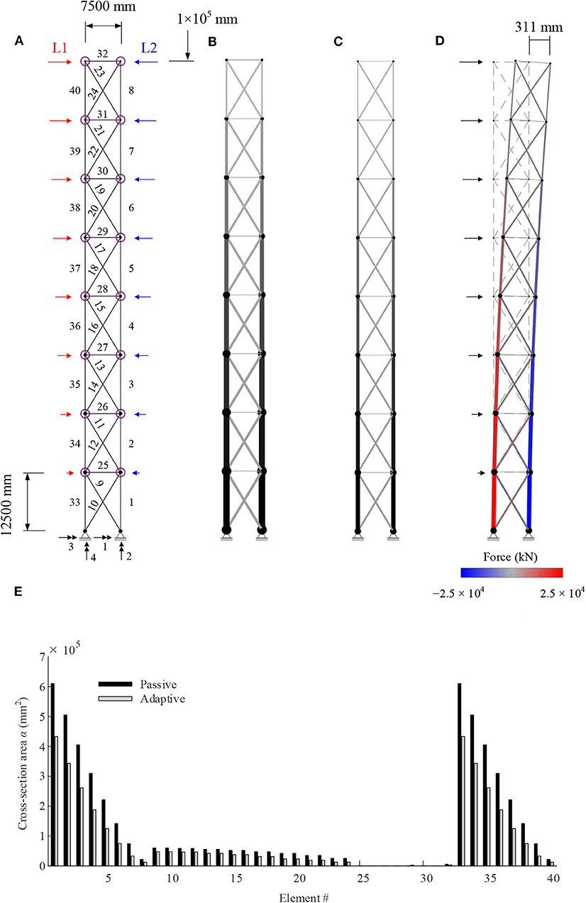
Figure 2. Multi-story building: (A) dimensions, controlled nodes, and loading; (B) passive; (C) adaptive (MUT 28%); (D) deformed shape and element forces of the adaptive solution under LC1 before control (magnification ×20); (E) element cross-section area passive vs. adaptive.
The structure is designed to support a permanent and a live load. The permanent load consists of self-weight (SW), which includes the weight of the actuators, and dead load (DL). The dead load is set to 2.94 kN/m2 (300 kg/m2) resulting in a uniformly distributed load of 22 kN/m (assuming 7.5 m of cover out of plane) applied every 4 m for each floor. The live loads, LL1 and LL2, are horizontally distributed in opposite direction (Figure 2A) with an intensity which is a function of the square root of the height to approximate a wind pressure distribution. The live-to-dead-load ratio is set to 1 and hence the live load maximum intensity is 2.94 kN/m2. The live load frequency of occurrence is modeled with a log-normal probability distribution (see section Step 3: Operational Energy Computation)
The adaptive solution is compared to a weight-optimized passive solution of identical topology subjected to the same loading and limit states. The passive solution has been optimized using a method given in Senatore et al. (2019) that produces similar results to the Modified Fully Utilized Design method (Patnaik et al., 1998). Figures 2B,C show the passive and adaptive solution, respectively. The optimal adaptive solution has been obtained for MUT = 28% (see Table 8). For the passive solution, the equivalent MUT = 13% thus showing that material is better utilized in the adaptive solution. Line thickness variation indicates the element diameter while the cross-section area is represented through a color gradient whereby a larger area is assigned a darker gray shade. The element cross-section area for both passive and adaptive solutions are also indicated by the bar chart shown in Figure 2E. With regard to the adaptive solution, elements #1, #33 and #25 have the largest and smallest diameter which are 1,707 and 100 mm, respectively. On average, the elements of the adaptive solution have a cross-section area and external diameter that are 45 and 23% smaller, respectively, with respect to the weight-optimized passive solution. Figure 2D shows the deformed shape of the adaptive solution under LC1 for the SLS case before control. As expected, the maximum deflection is 311 m which is above the serviceability limit (200 mm). The internal forces are indicated by color shading; red is for tension and blue for compression. Since the deformed shape under LC2 mirrors that under LC1, for brevity it is not illustrated.
The objective of this case study is to benchmark energy requirements between control strategies C1, C2, and C4. The configuration shown in Figure 2 (structure dimensions + loading) has been selected for this case study because it allows the application of control strategy C2. C2 can be only employed when displacement compensation is required but it is not necessary to control the forces because stress and stability limits are met without the contribution of the active system. The configuration selected for this case study met this condition for an MUT in the range 0 ≤ MUT ≤ 33%. In such range of the solution domain, which contains the optimal solutions for all cases considered in this study, the design for this configuration is purely stiffness governed thus allowing to benchmark control strategy C2 against C1 and C4.
The number of actuators for the different configurations are varied according to the conditions given for C1 and C2 (Table 2). For actuator configuration AC1 (only internal) three sub-cases are considered by decreasing the number of internal actuators from nact,int = ne to sint ≤ nact,int ≤ ne and finally to nact,int < sint. For AC2 (only external) the number of external actuators is set to the number of constrained degrees of freedom nact,ext = nsd = 4. For AC3 (combination of internal and external) two sub-cases are considered by setting the number of external actuators nact,ext = nsd = 4 (nact,ext > sext) and reducing the number of internal actuators from sint ≤ nact,int ≤ ne to nact,int < sint.
Tables 5–7 give results with regard to the metrics of interest for AC1, AC2, and AC3, respectively. The illustrations in Table 8 show the controlled shapes and the actuator layout for each configuration. In addition, labels indicate the actuators that are subjected to the most demanding control requirements including maximum force capacity and maximum length change/support displacement. For brevity, illustrations in Table 8 are only given for strategy C2 under load case LC1 (which is symmetrical to LC2).
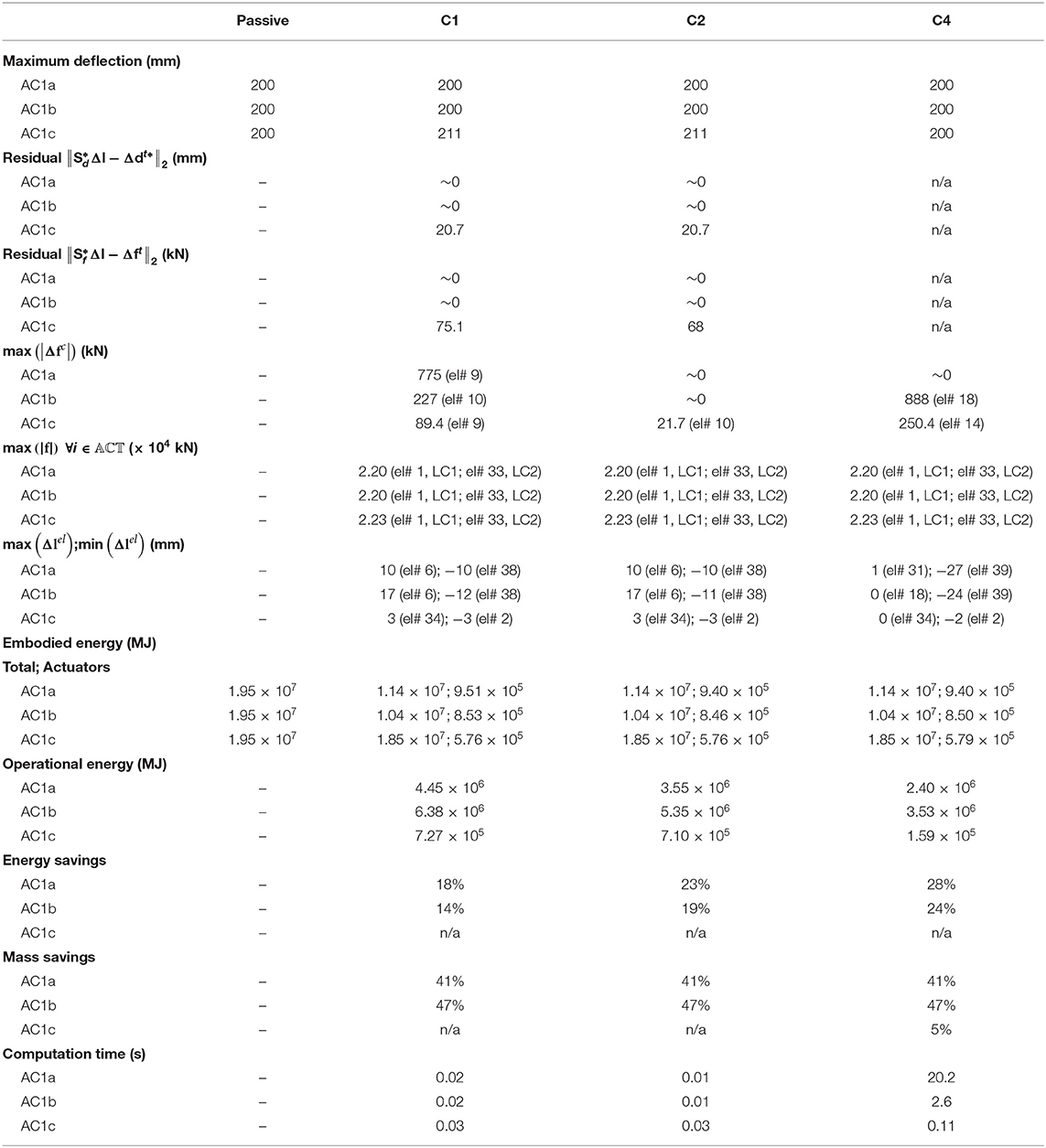
Table 5. AC1 results.

Table 6. AC2 results.
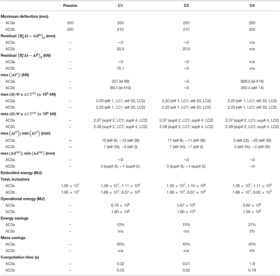
Table 7. AC3 results.
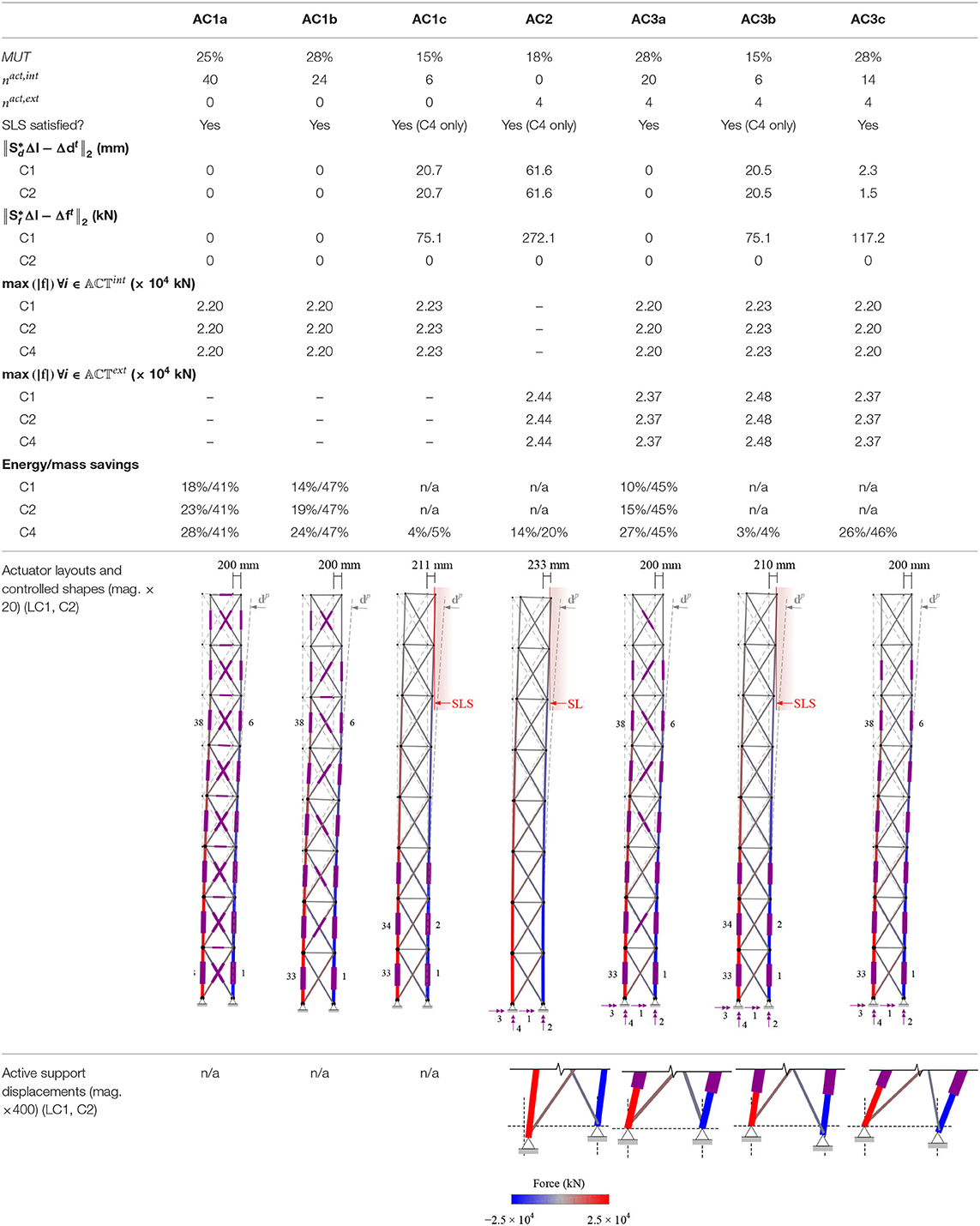
Table 8. Multi-story structure: summary of results.
AC1a: nact,int = ne
In this configuration all elements are active. The actuator commands for C2 are computed through Equation 25 (Table 2). The optimal design has been obtained for MUT = 25%.
For all control strategies, the maximum deflection max (|dp + Δdc − din|) (free-end) is reduced from 376 mm before control to 200 mm after control as required by SLS. Stress and stability limits are met through all control strategies. Good control accuracy is achieved through C1 and C2, as indicated by low residuals for force and shape control. In C4, control residuals are not computed because the target shape and forces are not supplied.
The largest force change max (|Δfc|) is required in C1 at element #9. This is because in C1 the forces are constrained to be equal to the target forces obtained through load-path optimization χ. Instead, shape control through C2 causes a zero change of forces. Control through energy minimization C4 also gives actuator commands that cause a minimum (practically zero) change of forces. The maximum force capacity max (|f|) is required in all strategies for the actuator placed at element #1 under LC1 and element #33 under LC2. The mass of the actuators subjected to maximum force capacity requirements is 2200 kg (see assumption given in section Material and Loading Assumptions). The maximum absolute length change is required in C4 for the actuator placed at element #39.
The actuation system embodied energy (and thus the mass) is on average 8% of the total (structure + actuation system) embodied energy among all control strategies. As expected, energy savings are the highest when the structure is controlled through C4. The operational energy for C4 is 53% of that required by C1. However, C2 is also efficient in terms of energy requirements. As expected, the computation time to obtain control commands through C4 is significantly higher than that required for C1 and C2.
AC1b: sint ≤ nact,int ≤ ne
In this configuration nact,int is set to nact,int = ncd + s = 24 which is the required number of actuators to obtain a unique solution for C1 [Section Control to Target Forces and Shapes (C1)]. Actuator commands for C2 are obtained through Equation 27 (Table 2). The optimal design has been obtained for MUT = 28%.
The maximum deflection max (|dp + Δdc − din|) is reduced from 415 mm before control to 200 mm after control through all strategies since the number of actuators meets the minimum requirement for accurate shape control. Low residuals indicate a good control accuracy through C1 and C2. Stress and stability limits are met through all control strategies.
Control strategy C4 requires the largest force change max (|Δfc|) at element #18. Control through C2 produces no change of forces while C4 causes a small force change compared to C1. The maximum force capacity max (|f|) is required in all strategies for the actuator placed at element 1 under LC1 and element 33 under LC2. The mass of the actuator subjected to maximum force capacity requirements is 2,200 kg. The maximum absolute length change is required in C4 for the actuator placed at element #39.
The actuation system embodied energy (and thus the mass) is on average 8% of the total (structure + actuation system) embodied energy among all control strategies. The computation time for C4 is lower than that in AC1a because the number of actuators is lower and thus the number of optimization variables (Equation 44 to 54) is reduced.
AC1c: nact,int < sint
In this configuration nact,int is set to 6, which is lower than the degree of internal static indeterminacy (sint = 7). Actuator commands for C2 are computed through Equations 28, 29 (Table 2). The optimal design has been obtained for MUT = 15%. The maximum deflection max (|dp + Δdc − din|) cannot be reduced from 260 mm to the serviceability limit (200 mm) because the number of actuators is significantly lower than the minimum requirement for accurate shape control. Control accuracy in AC1c is generally poor as indicated by higher control residuals than those given for AC1a and AC1b. Control residuals for C1 and C2 are similar, indicating a comparable performance for shape control through both strategies. Stress and stability limits are met through all control strategies.
The highest force change max (|Δfc|) is required by C4 at element #14. Since the number of actuators is lower than the minimum requirement to cause an impotent eigenstrain (Table 2), a relatively small change of force is also produced through C2. The maximum force capacity max (|f|) is required in C1, C2, and C4 for the actuator placed at element #1 under LC1 and element #33 under LC2. The mass of the actuator subjected to maximum force capacity requirements is 2,230 kg. The maximum absolute length change is required in C1 and C2 for the actuator placed at elements #34.
The actuation system embodied energy (and thus the mass) is on average 3% of the total (structure + actuation system) embodied energy among all control strategies. Since SLS has not been met for this configuration in C1 and C2, energy and mass savings are not given.
In this configuration, there are no internal actuators and all supports are set to active nact,ext = 4. Actuator commands for C2 are computed through Equation 27 (Table 2). The optimal design has been obtained for MUT = 18%. The maximum deflection max (|dp + Δdc − din|) can be reduced from 260 mm to the serviceability limit (200 mm) through C4, but not C1 or C2. Control accuracy in AC2 is generally poor for C1 and C2 as indicated by higher control residuals than those given for AC1. Control residuals for C1 and C2 are identical, indicating a comparable performance for shape control. Stress and stability limits are met through all control strategies.
The highest force change max (|Δfc|) is required in C1 at element #9. Since the number of actuators is higher than the degree of external indeterminacy nact,ext > sext, it is possible to produce an impotent eigenstrain through C2 and thus there is no change of forces. The active supports provide a force couple that opposes the action of the external load. Under LC1, the vertical displacements are opposite (upward for support 2 and downward for support 4) (see illustration in Table 8). Identical but opposite in sign is the reaction of the active supports under LC2. The maximum force capacity max (|f|) is required in C1 and C2 for the actuator placed at support 2 (vertical direction) under LC1 and support 4 (vertical direction) under LC2. The mass of the actuators subjected to maximum force capacity requirements is 2,440 kg. The maximum absolute displacement is required in C1 for the external actuator placed at support #3 (horizontal direction).
The actuation system embodied energy (and thus the mass) is on average 2% of the total (structure + actuation system) embodied energy among all control strategies. Since SLS has not been met for this configuration in C1 and C2, energy and mass savings are not given.
AC3a: sint ≤ nact,int ≤ ne, nact,ext = 4
In this configuration nact is set to nact = ncd + s = 24 which is the required number of actuators to obtain a unique solution for C1. In this case nact = nact,int + nact,ext where nact,int = 20 and nact,ext = 4. Actuator commands for C2 are computed through Equation 27 (Table 2). The optimal design has been obtained for MUT = 28%. The maximum deflection max (|dp + Δdc − din|) is reduced from 415 mm to within serviceability limits (200 mm) for all strategies. Stress and stability limits are met through all control strategies. Control residuals are relatively low, indicating a good control accuracy for C1 and C2. Shape control residuals for C2 are lower than those for C1.
Control strategy C4 requires the largest force change max (|Δfc|) at element #18. The change of force in C1 is lower than that in C4. Control through C2 instead produces no change of forces. The maximum force capacity max (|f|) is required in all strategies for the actuators placed at element #1 and support #2 under LC1 and element #33 and support #4 under LC2. The mass of the actuators subjected to maximum force capacity requirements is 2,200 kg for the internal type and 2370 kg for the external one. The maximum absolute length change is required in C4 for the internal actuator placed at element #39. The active support displacements are practically zero for all strategies hence no action is required for the external actuators.
The actuation system embodied energy (and thus the mass) is on average 10% of the total (structure + actuation system) embodied energy among all control strategies. The energy savings are the highest for C4, which requires only 53% of the operational energy required by C1. Due to high force requirements that result in large operational energy consumption, the active supports do not contribute to displacement control in C4 i.e., control commands for the external actuators obtained through C4 are practically zero. As for previous cases, the computation time required by C4 is significantly higher than that for C1 and C2.
AC3b: nact,int < sint, nact,ext = 4
In this configuration nact = nact,int + nact,ext = 10 where nact,int = 6 and nact,ext = 4. Actuator commands for C2 are obtained through Equations 28, 29 (Table 2). The optimal design is obtained for MUT = 15%. The maximum deflection max (|dp + Δdc − din|) can be reduced from 260 mm to the serviceability limit (200 mm) through C4, but not C1 and C2.
Control strategy C4 requires the largest force change max (|Δfc|) at element #14. Control through C2 instead produces no change of forces because the total number of actuators is nact > s (Table 2). The maximum force capacity max (|f|)is required in all strategies for the actuators placed at element #1 and support #2 under LC1 and element #33 and support #4 under LC2. The mass of the actuators subjected to maximum force capacity requirements is 2,230 kg for the internal type and 2,480 kg for the external one. The maximum absolute length change is required in C1 and C2 for the internal actuator placed at element #34. The maximum absolute displacement is required in C1 and C2 for the external actuator placed at support #2 (vertical direction).
The actuation system embodied energy (and thus the mass) is on average 5% of the total (structure + actuation system) embodied energy among all control strategies. Since SLS has not been met for this configuration in C1 and C2, energy and mass savings are not given.
A comparison of the results obtained for configurations AC1, AC2 and AC3 is given in Table 8. The actuator placement and controlled shapes under LC1 are illustrated for each configuration. For brevity, only the configurations for C2 are illustrated. The internal actuators are represented by thicker lines placed in the middle of the elements while the external actuators are represented by arrows placed in proximity of the supports.
Generally, accurate control is only possible through C4 if the number of internal actuators is lower than the degree of internal static indeterminacy nact,int < sint. For this case study, the external actuators are not as effective as the internal ones. In AC2, although all supports are active, the SLS limit could only be met through C4, but not C1 and C2. Control accuracy improves when external actuators are employed in combination with a sufficient number of internal actuators nact,int > sint (AC3a).
The actuation system embodied energy (and thus the total mass of the actuators) is only a fraction of the total embodied energy (structure + actuation system). The actuation system is AC3a embodies the highest energy which, nonetheless, is only 10% of the total embodied energy for this configuration.
For all configurations, C4 produces solutions with the lowest operational energy requirement. However, since C4 is based on a non-convex optimization that employs explicit constraints on displacements, the computation time to obtain control commands is on average 2,020 times higher than that required for C1 and C2. C2 is also efficient with regard to operational energy requirement which is always lower than that required by C1. Note that C2 can be employed when displacement compensation is required but it is not necessary to control the forces because stress and stability limits are met without the contribution of the active system.
Operational energy requirements when using external actuators are generally higher, which results in lower energy and mass savings for AC3a compared to AC1b. In AC3a (nact,int = 20, nact,ext = 4) using control strategy C4, the combination of internal and external actuators produce a small increase (3%) of the energy savings with respect to AC1b (nact,int = 24) at the cost of a marginal reduction of mass savings (2%). This is because generally, the maximum force capacity of external actuators is higher than that of internal actuators.
A parametric study has been carried out to evaluate the sensitivity of energy requirements, as well as mass and energy savings, with respect to the number of internal actuators nact,int. An adaptive structure solution has been obtained for each configuration by setting MUT = 28%, which is kept constant. The number of internal actuators nact,intvaries from nact,int = neto nact,int = sint while the number of external actuators is kept constant nact,ext = ncd = 4. The control strategy adopted in this parametric study is C4. Figure 3 shows (a) the variation of energy requirements as well as (b) energy and mass savings with respect to nact,int. The embodied energy (and thus the mass) remains almost constant because the MUT is kept constant. The slight increase of embodied energy with the number of actuators is due to the increase of the actuation system embodied energy. Operational energy requirements increase as nact,int reduces from nact,int = ne; conversely, energy savings decrease. However, energy savings decrease significantly only after the number of internal actuators is further reduced from nact,int = 14. This configuration is denoted as AC3c. Metrics of interest for AC3c are given in Table 8 which includes an illustration of the actuator placement and controlled shape obtained through C2 under LC1. AC3c can be regarded as the best overall configuration because it achieves very similar energy and mass savings to AC3a (which has the highest energy savings), albeit using 30% fewer actuators.
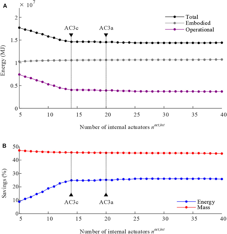
Figure 3. Multi-story structure: (A) total, embodied, and operational energy; (B) energy and mass savings vs. the number of internal actuators.
The arch truss considered in this study can be thought of as an arch bridge reduced to two dimensions. The geometry of the structure is illustrated in Figure 4A which shows dimensions, support and loading conditions. The vertical displacement of all free nodes of top and bottom chords are set as controlled degrees of freedom for a total of ncd = 19. The controlled nodes are indicated by circles. The serviceability limit is set to S/1,000 = 100 mm, where S = 100 m is the span of the bridge. The degree of static indeterminacy (s) is sint = 0 internally and sext = 3 externally. The structure is designed to support a permanent and a live load. The permanent load consists of self-weight (SW), which includes the weight of the actuators, and dead load (DL). The dead load (DL) is uniformly distributed on the top chord nodes with an intensity of 10 kN/m. There are three uniformly distributed live loads (LL) cases. LL1 is applied on the whole span while LL2 and LL3 are applied on one-half of the span. The live-to-dead-load ratio is set to 1 for LL1 to simulate normal traffic conditions and to 1.25 for LL2 and LL3 to simulate asymmetric loadings due to vehicular traffic. The live load frequency of occurrence is modeled with a log-normal probability distribution (see section Step 3: Operational Energy Computation).
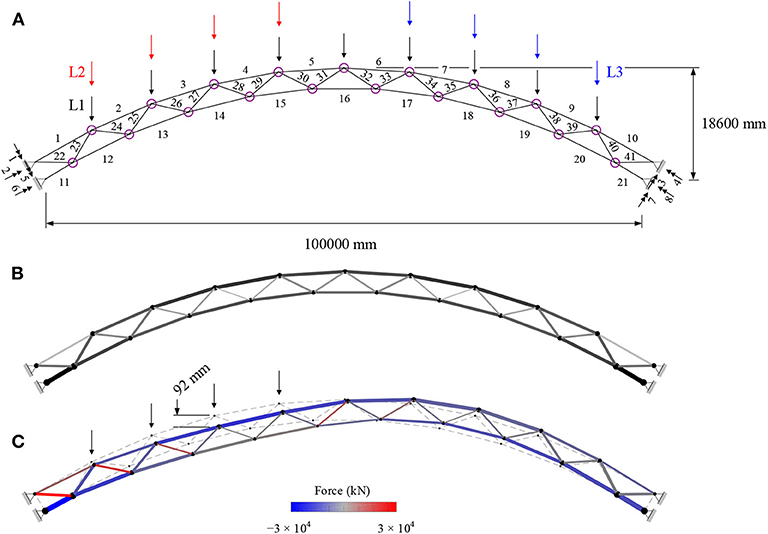
Figure 4. Arch bridge: (A) dimensions, controlled nodes, and loading; (B) adaptive; (C) deformed shape and element forces under LC2 before control (magnification × 20).
Figure 4B shows the adaptive solution which has been obtained for MUT = 68%. Element diameters are indicated by line thickness variation, cross-section areas and element forces are indicated by color shading as for the previous case study (Section High-Rise Structure). Elements #11, #21 and #28, #35, #42, #43 have the largest and smallest diameter, which are 1,210 and 200 mm, respectively. Figure 4C shows the deformed shape under LC2 (before control). The maximum nodal displacement is 92 mm, which is lower than the required serviceability limit (100 mm), hence there is no need for active compensation of displacements. For this reason, the focus of this study will be on force control through strategy C3 i.e., nilpotent eigenstrain. In this case, the control objective is to maintain an optimal load-path under multiple load cases without causing any (or minimal) change of the node positions. Since the structure works as an arch bridge, an optimal load-path is when both top and bottom chords work in compression even under asymmetric loading. The target forces Δft are obtained through process χ (Section Step 1: Embodied Energy Optimization) by adding extra constraints that limit the forces in the top and bottom chord elements to compression.
The number of actuators for the different configurations are varied according to the conditions given in Table 3. For actuator configuration AC1 (only internal) three sub-cases are considered by decreasing the number of internal actuators from nact,int = ne to ncd < nact,int ≤ ne and finally to nact,int ≤ ncd. For AC2 (only external) the number of external actuators is set to the number of constrained degrees of freedom nact,ext = nsd. For AC3 (combination of internal and external) two sub-cases are considered by setting the number of external actuators nact,ext = nsd (nact,ext > sext) and reducing the number of internal actuators from nact,int > s + ncd to nact,int < s + ncd.
Control strategy C3 is benchmarked against C4. For both strategies, the change of forces Δf = Δfp + Δfc should be such that all elements of top and bottom chords are in compression under all load cases. Control accuracy is evaluated through a measure of the maximum change of displacements which should be as small as possible i.e., max (|Δdc|) ≈ 0. Results for AC1 to AC3 are summarized in Table 9. Each configuration is illustrated in Figure 5, which shows the actuator layout, element forces and controlled shapes.
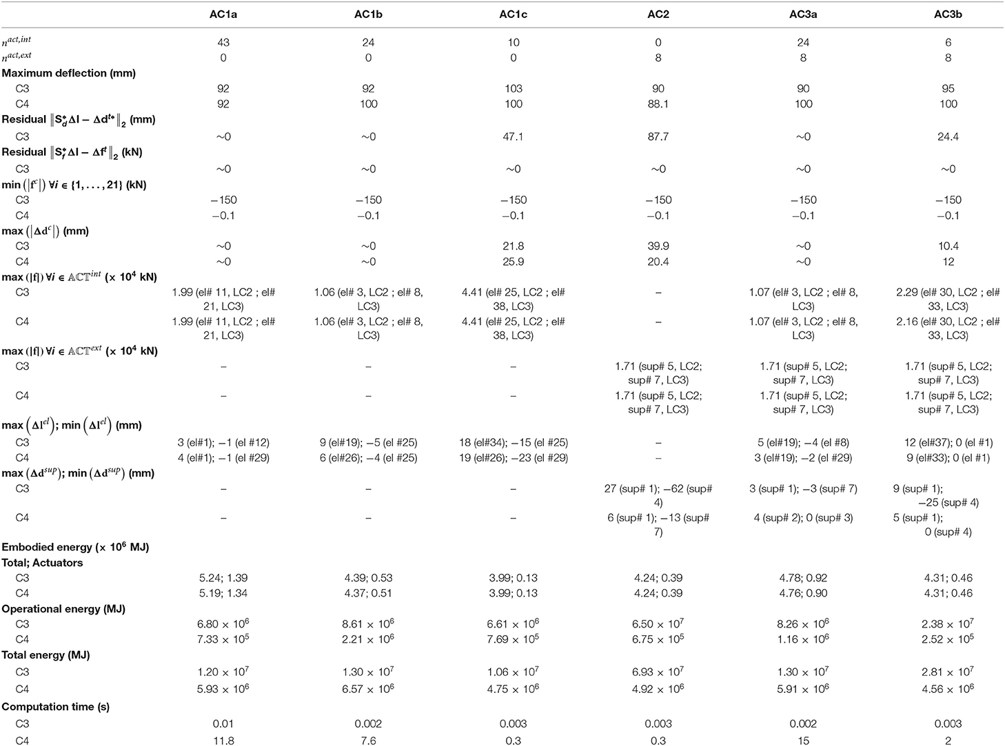
Table 9. Arch bridge: summary of results.
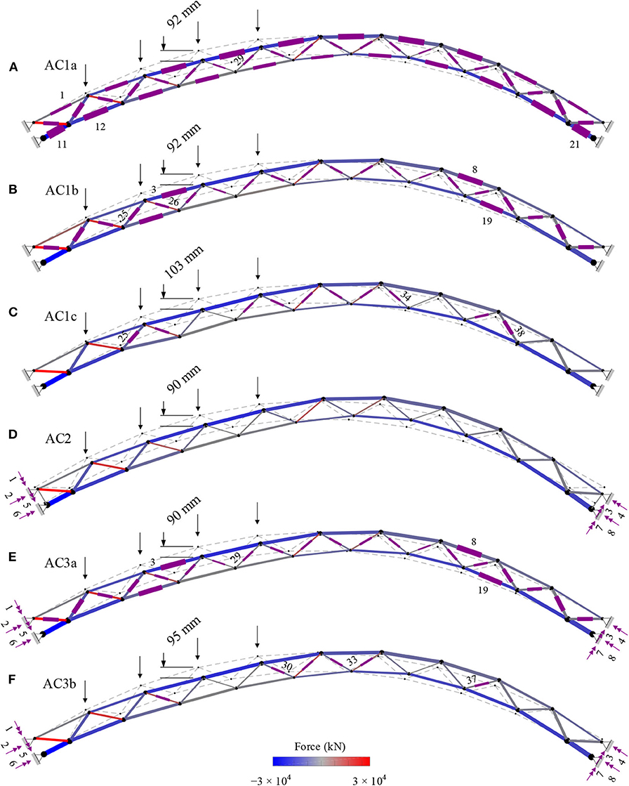
Figure 5. Arch bridge: actuator layout, element forces, and controlled shapes (magnification × 20) under LC2 for AC1a-c (only internal actuators), AC2 (only external actuators) and AC3a-b (combination of internal and external actuators).
In AC1a, since all elements are set to active (43 actuators, Figure 5A) control commands for C3 are obtained through Equation 35. Both strategies produce actuator commands that cause a nilpotent eigenstrain and top and bottom chord elements are controlled in compression under all load cases. Accurate force control for C3 is indicated by low residuals . The operational energy for C4 is 11% of that required by C3. the computation time to obtain control commands through C4 is significantly higher than that required for C3.
In configuration AC1b, nact,int = 24 > s + ncd (Figure 5B). Similar to AC1a, it is possible to obtain control commands that do not cause any change of node positions and to control the internal forces so that all elements of top and bottom chords are in compression. The operational energy for C4 is 26% of that required by C3. Similar to AC1a, the computation time for C4 is significantly higher than that for C3.
In AC1c, nact,int = 10 (Figure 5C). In this case, it is not possible to obtain control commands that do not cause any change of node positions through neither C3 nor C4. Control strategy C3 requires a change of node position max (|Δdc|)= 21.8 mm which results in a violation of the serviceability limit (100 mm). As indicated by high residuals , control accuracy is poor due to the low number of actuators employed in this configuration. Through both strategies, top and bottom chord elements are controlled in compression under all load cases. The operational energy for C4 is 12% of that required by C3. In AC1c, the computation time is significantly lower than that required in configurations with more actuators such as AC1a and AC1b.
In AC2, all supports are set to active for a total of nact,ext = 8 (Figure 5D). In this case, it is not possible to obtain control commands that do not cause any change of node positions through neither C3 nor C4. As discussed in section Force Control Through Nilpotent Eigenstrain (C3), the effect of an active support is to move the node positions and therefore it cannot be employed to produce a nilpotent eigenstrain. Although the serviceability limit (100 mm) is still respected, control strategy C3 requires the largest change of node position max (|Δdc|) of 39.9 mm. Similar to AC1c, high residuals indicate poor control accuracy. Similar to AC1c, top and bottom chords are in compression under all load cases through both control strategies. The operational energy for C4 is only 1% of that required by C3. In AC2, the computation time is comparable to AC1c.
In AC3a and AC3b, all supports are set to active for a total of nact,ext = 8 in combination with nact,int = 24 > s + ncd and nact,int = 6 internal actuators (Figures 5E,F). When nact,int < ne or when the supports are active (AC2, AC3a, and AC3b) control commands are computed through Equations 38 and 39, which produce an approximate nilpotent eigenstrain. No significant change of shape occurs in AC3a for both C3 and C4, while in AC3b it is not possible to obtain control commands that do not cause any change of node positions through neither C3 nor C4. Although the serviceability limit (100 mm) is still respected in AC3b, control strategy C3 requires the largest change of node position max (|Δdc|)= 10.4 mm. High residuals in AC3b indicate poor control accuracy due to the low number of actuators. In both AC3a and AC3b, and with both control strategies, top and bottom chords are in compression under all load cases. The operational energy for C4 is only 14% and 1% of that required by C3 in AC3a and AC3b, respectively.
The largest change of node positions occurs in AC2, where the actuators are only placed at the supports. No change of node positions occurs in AC1a, AC1b, and AC3a where the number of actuators nact = 24 > s + ncd satisfies the condition to obtain a unique solution with low residuals for C1, C2, and C3 (see section Control Through Impotent and Nilpotent Eigenstrain).
The maximum force capacity max (|f|)is required in AC1c for the actuators placed at element #25 and #38 under LC2 and LC3, in AC2, AC3a, and AC3b for the actuators placed at support #5 and 7 under LC2 and LC3. The mass of the actuators subjected to maximum force capacity requirements is 4,410 kg for the internal type and 1710 kg for the external one. The maximum absolute length change is required for the actuator placed at element #34 in AC1c where the number of internal actuators is the lowest. Generally, the active supports move inward to counteract the effect of the external load as shown in Figure 5D for AC2. The maximum absolute support displacement occurs in AC2 for the external actuator placed at support #4.
In all configurations and under all load cases, top and bottom chords are controlled to stay in compression. Accurate force control in C3 is indicated by the residual , which is practically zero for all cases (Table 9) including AC2 where only active supports are employed. Figure 6 shows a bar chart of the internal forces for top and bottom chord elements #1 to #21 before control (black), after control through C3 (light gray) and after control through C4 (dark gray). For brevity, only forces for load case LC2 and configuration AC1b are given. The maximum force after control through C3 among the top and bottom chord elements, max (fc) ∀i ∈ {1, …, 21}, is −150 kN in all configurations. The maximum force after control through C4 among the top and bottom chord elements, max (fc) ∀i ∈ {1, …, 21}, is −0.1 kN in all configurations.
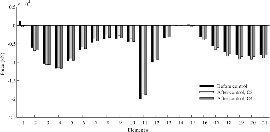
Figure 6. Arch bridge: internal forces in the top and bottom chord elements for AC1b under LC2.
The embodied energy (and thus the mass) is lower for AC1c, AC2, and AC3b compared to the other configurations, which employ more actuators. This is because in AC1a, AC1b, and AC3a, actuators are placed on elements subjected to high forces such as element #11, #21, #3, #8, #13 and #19, which causes the actuation system embodied energy to reach 27%, 12% and 20% of the total (structure + actuation system) embodied energy, respectively. For AC1c, AC2 and AC3b instead, the actuation system embodied energy is 3, 9, and 10% of the total embodied energy.
Through strategies C3 and C4, the structure is controlled as required so that top and bottom chords are in compression even under asymmetrical load cases. Both strategies produce actuator commands that generally cause a minimal change of shape, which, in this case, was not needed as deflection limits are met without the contribution of the active system. The computation time to obtain a solution through C4 is on average 1,180 times higher than that required by C3. However, control through C4 requires significantly less operational energy which is on average only 9% of that required by C3.
Operational energy requirements are the highest in AC2 through C3 because the external actuators are required to work against high forces and to perform larger displacements compared to those required by the other configurations. Combination of internal and external actuators in AC3a is effective to reduce the operational energy requirement with respect to AC1b without reducing shape control accuracy (the maximum change of node positions and shape control residuals are practically zero for AC1b and AC3a). Configuration AC3b (nact,int = 6, nact,ext = 8) is the best overall configuration because its embodied energy (and thus the mass) is only 8% higher than that of the minimum embodied energy configuration (AC1c) and its operational, as well as total energy, are the lowest among all configurations. In addition, AC3b employs fewer actuators compared to other configurations e.g. 43 actuators in AC1a, 24 in AC1b, 32 in AC3a vs. 14 actuators in AC3b.
Closed-form solutions to decouple force and shape control through impotent and nilpotent eigenstrain have been presented through strategies C2 and C3. Within the assumption of small deformations, impotent (C2) and nilpotent (C3) eigenstrain can be caused through actuation exactly (Δfc = 0;Δdc* = 0, respectively) provided that the null space of the force and shape influence matrices exist. The nullity of is greater than zero if the number of actuators is higher than the degree of static indeterminacy i.e. sext < nact,ext ∪ sint < nact,int; the nullity of is greater than zero if the number of internal actuators is higher than the number of controlled degrees of freedom i.e., nact,int > ncd. When these conditions are met, generally, force and shape control can be decoupled i.e., forces can be controlled without changing the shape through a nilpotent eigenstrain (Δfc ≈ Δft; Δdc* = 0) and the shape can be controlled without changing the forces through an impotent eigenstrain (Δfc = 0;Δdc* ≈ Δdt). In some cases, depending on the actuator layout and the position of the controlled degrees of freedom, the basis of the null space of the force and shape influence matrices may be ill-conditioned. In such cases, and when the number of actuators does not meet required conditions (Tables 2, 3), control commands to cause an approximate impotent and nilpotent eigenstrain can be obtained through optimization as shown in section Shape Control Through Impotent Eigenstrain (C2) and Force Control Through Nilpotent Eigenstrain (C3), respectively. Note that it is not possible to obtain actuator commands that cause an exact (Δdc* = 0) nilpotent eigenstrain when active supports are employed i.e., nact,ext > 0. In such case, nilpotent eigenstrain can only be approximated through optimization in order to control the forces as required albeit causing a small change of shape.
The structure-control optimization method given in Senatore et al. (2019) combined with the control strategies presented in section Control Strategies has been applied to the design of a high-rise structure and an arch bridge to benchmark control accuracy and energy requirements. Actuator layouts that include active elements (internal actuators), active supports (external actuators) and combination of both have been tested. For all control strategies, the actuator placement has been obtained through the method given in Senatore et al. (2019) and control commands are obtained so that that ULS and SLS are respected. Information regarding control requirements in terms of actuator maximum force capacity and length change has also been given for each configuration.
Since C4 is based on a non-convex optimization problem, the computation time to obtain control commands is significantly higher than that required for C1, C2, and C3. C1, C2, and C3 are convex problems that comprise either constrains on forces or displacements but not simultaneously and thus an approximate solution can be obtained in lower computation time. Owing to the simplicity and computational efficiency of C1 and C2, they have been successfully applied to linear (Senatore et al., 2018c) and geometric non-linear (Reksowardojo et al., 2020b) real-time control of experimental adaptive structures equipped with linear actuators.
The operational energy required by C2 and C4 is lower than that required by C1. Control through C1 aims to cause a prescribed change of forces and node positions and thus it involves more stringent constraints with respect to C4 in which forces and displacements are only constrained as required by ULS and SLS, respectively. This is the main reason C1 requires larger operational energy with respect to C2 and C4. While C4 always requires the least energy, C2 has comparable operational energy requirements. In addition, C2 is significantly more efficient in computation time terms which is on average 0.05% with respect to C4. That being said, C2 can only be employed when displacement compensation is required but it is not necessary to control the forces because stress and stability limits are met without the contribution of the active system. In these conditions, shape control through impotent eigenstrain (C2) should be employed instead of C1 or C4. This is an important finding because, since high-intensity loads occur rarely, it is only necessary to reduce displacements within SLS limits without affecting the internal forces under most occurrences of the load probability distribution which are above the load activation threshold (LAT) (see section Step 3: Operational Energy Computation). This is particularly relevant to stiffness governed structures for which non-controlled displacements are likely to violate SLS limits before any critical stress condition might occur. In addition, when fail-safe constraints that account for control system failure and power breakdown are added to the structural optimization process outlined in section Synthesis of Minimum Energy Adaptive Structures (Senatore et al., 2019; Wang and Senatore, 2020), ULS is met without the contribution of the active system and thus only displacement compensation is required under SLS load cases.
In general, external actuators require higher operational energy than internal actuators since forces acting on the supports are usually higher than the element forces. However, a layout that combines external and internal actuators may require lower operational energy compared to one which comprises only internal actuators. For example, for the arch bridge case study, simulations have shown that it is effective to use external actuators in combination with internal actuators to lower the control energy.
A parametric study has been carried out to evaluate the sensitivity of energy requirements, as well as mass and energy savings, with respect to the number of internal actuators nact,int. Embodied (and thus material mass) and operational energy requirements increase as nact,intreduces from nact,int = ne. Conversely, mass and energy savings decrease. However, mass and energy savings decrease significantly only when the number of internal actuators is significantly lower than nact = s + ncd(static indeterminacy+ controlled degrees of freedom), which is the condition to obtain a unique solution with low residuals for C1, C2, and C3 (see section Control Strategies).
This work has presented the formulation of four control strategies for adaptive structures equipped with linear actuators: (C1) force and shape control to obtain prescribed changes of forces and node positions; (C2) shape control through impotent eigenstrain when displacement compensation is required without affecting the forces; (C3) force control through nilpotent eigenstrain when displacement compensation is not required and (C4) force and shape control through operational energy minimization. These control strategies have been integrated within a previously developed structure-control optimization method (Senatore et al., 2019) which produces adaptive structural configurations that outperform equivalent weight-optimized passive structures on a variety of aspects: the adaptive solutions embody a significantly reduced material mass, they can be much more slender, they have a higher stiffness because deflections are controlled within tight limits, they are minimum energy solutions thus reducing environmental impacts.
The main contributions of this work are: (1) formulation of three new control strategies C2, C3 and C4 which extend the integrated structure-control optimization method given in Senatore et al. (2019); (2) derivation of closed-form solutions and formulation of optimization methods to decouple force and shape control through nilpotent and impotent eigenstrain; (3) extension of the force and shape control formulation given in Senatore et al. (2019), which considered only internal actuators (i.e., active elements), to include the action of external actuators placed at supports (i.e., active supports).
The following conclusions are drawn from the analytic and numerical studies presented in this paper:
• A necessary condition to decouple force and shape control is the existence of the null space of the force and shape influence matrices defined in Force and Shape Influence Matrices. Therefore, it follows that: (1) the shape can be controlled as required without changing the forces through an impotent eigenstrain if the number of actuators is higher than the degree of static indeterminacy i.e., sext < nact,ext ∪ sint < nact,int; (2) forces can be controlled as required without changing the shape through a nilpotent eigenstrain if the number of internal actuators is higher than the number of controlled degrees of freedom i.e., sext < nact,ext ∪sint < nact,int.
• Energy savings increase as the number of actuators increases from nact = s. However, no further significant savings are gained as the number of actuators increases from nact = s + ncd that is the sum of the degree of static indeterminacy and the number of controlled degree of freedom.
• When displacement compensation is required but no change of forces is needed, shape control through impotent eigenstrain (C2) is an effective strategy. C2 has comparable energy requirements to C4, which produces control solutions of minimum energy, and it is significantly more efficient than C4 with regard to computation time.
Future work could look into applying the methods formulated in this paper to other structural configurations with the aim to evaluate in which conditions the interaction of internal and external actuators is most beneficial in energy/mass savings terms as well as to increase structural performance for example of slender high-rise structures or long-span bridges. In this work, actuators are assumed to be installed in series, and thus they have to carry the full force in the corresponding element. Another approach is to consider the actuators in parallel with the elements thereby decoupling the active elements from load transfer (Weidner et al., 2018; Böhm et al., 2020). This approach could be beneficial for control through nilpotent eigenstrain where the main objective is force control. Future work could extend the design and control strategies given in this paper to consider actuators installed in parallel. Extensions of the control strategies presented in this work to include geometric non-linear shape control (Reksowardojo et al., 2020a) as well as consideration of dynamics could also be subject of future investigations.
The raw data, including source code, which supports the conclusions of this article will be made available by the authors, without undue reservation. For up to date contact information visit http://www.gennarosenatore.com.
GS set up research objectives and directions. Method implementation was carried out by AR and GS. AR carried out simulations and wrote the first draft of the paper with GS actively involved in the rest of the writing process. All authors contributed to the manuscript revision, and reviewed and approved the final version.
The authors thankfully acknowledge the Swiss National Science Foundation who provided core funding for this research via project 200021_182033 (Structural Adaptation through Large Shape Changes).
The authors declare that the research was conducted in the absence of any commercial or financial relationships that could be construed as a potential conflict of interest.
Achtziger, W. (2007). On simultaneous optimization of truss geometry and topology. Structural and Multidisciplinary Multidisc. Optimization. 33, 285–304. doi: 10.1007/s00158-006-0092-0
Begg, D. W., and Liu, X. (2000). On simultaneous optimization of smart structures - part II: algorithms and examples. Comput. Methods Appl. Mech. Eng. 184, 25–37. doi: 10.1016/S0045-7825(99)00317-5
Bekker, P. C. F. (1982). A life-cycle approach in building. Build. Environ. 17, 55–61. doi: 10.1016/0360-1323(82)90009-9
Böhm, M., Steffen, S., Geiger, F., Sobek, W., Bischoff, M., and Sawodny, O. (2020). “Input modeling for active structural elements – extending the established FE-Workflow for modeling of adaptive structures,” in International Conference on Advanced Intelligent Mechatronics, (Boston, MA).
Böhm, M., Wagner, J., Steffen, S., Sobek, W., and Sawodny, O. (2019). “Homogenizability of element utilization in adaptive structures,” in 15th International Conference on Automation Science and Engineering (CASE), (Vancouver, BC). doi: 10.1109/COASE.2019.8843066
Casciati, F., Rodellar, J., and Yildirim, U. (2012). Active and semi-active control of structures - theory and applications: a review of recent advances. J. Intell. Mater. Syst. Struct. 23, 1181–1195. doi: 10.1177/1045389X12445029
Cole, R. J., and Kernan, P. C. (1996). Life-cycle energy use in office buildings. Build. Environ. 31, 307–317. doi: 10.1016/0360-1323(96)00017-0
ENERPAC (2016). E328e Industrial Tools - Europe. Available online at: http://www.enerpac.com/en-us/downloads. (accessed December 07, 2017).
Frohlich, B., Gade, J., Geiger, F., Bischoff, M., and Eberhard, P. (2019). Geometric element parameterization and parametric model order reduction in finite element based shape optimization. Computational Comput. Mechanics. 63:, 853.–868. doi: 10.1007/s00466-018-1626-1
Haftka, R. (1985). Simultaneous analysis and design. AIAA Journal. 23, 1099–1103. doi: 10.2514/3.9043
Hammond, G. P., and Jones, C. I. (2008). Embodied energy and carbon in construction materials. Proceedings of the Institution of Civil Engineers-. Energy. 161, 87–98. doi: 10.1680/ener.2008.161.2.87
Irschik, H., and Ziegler, F. (2001). Eigenstrain without stress and static shape control of structures. AIAA Journal. 39, 1985–1990. doi: 10.2514/2.1189
Kaethner, S., and Burridge, J. (2012). Embodied CO2 of structural frames. The Structural. Engineer. 90, 33–40.
Lu, L. Y., Utku, S., and Wada, B. (1992). On the placement of active members in adaptive truss structures for vibration control. Smart Materials and Structures. 1, 8–23. doi: 10.1088/0964-1726/1/1/003
Neuhaeuser, S., Weickgenannt, M., and Witte, C. (2013). Stuttgart SmartShell – a full scale prototype of an adaptive shell structure. J. of the International Association for Shell and Spatial Structures. 548, 259–270.
Nyashin, Y., Lokhov, V., and Ziegler, F. (2005). Decomposition method in linear elastic problems with eigenstrain. Journal of Applied Appl. Mathematics and Mechanics. 85, 557–570. doi: 10.1002/zamm.200510202
Patnaik, S. (1973). An integrated force method for discrete analysis. Int. J. Numer. Methods Eng. 6, 237–251. doi: 10.1002/nme.1620060209
Patnaik, S., Gendy, A., Berke, S., and Hopkins, D. (1998). Modified Fully Utilized Design (MFUD) method for stress and displacement constraints. International Int. Journal for Numerical Numer. Methods in Engineering. 41, 1171–1194.
Pellegrino, S. (1990). Analysis of prestressed mechanisms. Int. J. Solids Struct. 26, 1329–1350. doi: 10.1016/0020-7683(90)90082-7
Pellegrino, S. (1993). Structural computations with the singular value decomposition of the equilibrium matrix. International Int. Journal of Solids and Structures. 30, 3025–3035. doi: 10.1016/0020-7683(93)90210-X
Pellegrino, S., and Calladine, C. (1986). Matrix analysis of statically and kinematically indeterminate frameworks. International Int. Journal of Solids and Structures. 22, 409–428. doi: 10.1016/0020-7683(86)90014-4
Ramesh, A. V., and Utku, S. (1991). Real-time control of geometry and stiffness in adaptive structures. Comput. Methods Appl. Mech. Eng. 90, 761–779. doi: 10.1016/0045-7825(91)90183-7
Reinhorn, A. M., Soong, T. T., Riley, M. A., and Lin, R. C. (1993). Full-scale implementation of active control. II: installation and performance. Journal of Structural Struct. Engineering. 119, 1935–1960. doi: 10.1061/(ASCE)0733-9445(1993)119:6(1935)
Reksowardojo, A., Senatore, G., Srivastava, A., Smith, I. F. C., Unterreiner, H., and Carroll, C. (2020b). “Design and control of a prototype structure that adapts to loading through large shape changes,” in Proceedings of the 21st International Federation of Automatic Control World Congress, (Berlin).
Reksowardojo, A. P., and Senatore, G. (2020). A proof of equivalence of two force methods for active structural control. Mech. Res. Commun. 103:103465. doi: 10.1016/j.mechrescom.2019.103465
Reksowardojo, A. P., Senatore, G., and Smith, I. F. C. (2019). Experimental testing of a small-scale truss beam that adapts to loads through large shape changes. Frontiers in Built Environment. 5:93. doi: 10.3389/fbuil.2019.00093
Reksowardojo, A. P., Senatore, G., and Smith, I. F. C. (2020a). Design of structures that adapt to loads through large shape changes. Journal of Structural Struct. Engineering (ASCE). 146:04020068. doi: 10.1061/(ASCE)ST.1943-541X.0002604
Röck, M., Saade, M. M., Balouktsi, M., Rasmussen, F. R., Birgisdottir, H., Frischknecht, R., et al. (2020). Embodied GHG emissions of buildings - the hidden challenge for effective climate change mitigation. Appl. Energy. 258:114107. doi: 10.1016/j.apenergy.2019.114107
Rodellar, J., Mañosa, V., and Monroy, C. (2002). An active tendon control scheme for cable-stayed bridges with model uncertainties and seismic excitation. Structural Struct. Control and Health Monitoring. 9, 75–94. doi: 10.1002/stc.4
Senatore, G., Duffour, P., and Winslow, P. (2018a) Energy and cost analysis of adaptive structures: case studies. Journal of Structural Struct. Engineering Eng. (ASCE). 144:04018107. doi: 10.1061/(ASCE)ST.1943-541X.0002075
Senatore, G., Duffour, P., and Winslow, P. (2018b). Exploring the application domain of adaptive structures. Engineering Eng. Structures. 167, 608–628. doi: 10.1016/j.engstruct.2018.03.057
Senatore, G., Duffour, P., and Winslow, P. (2019). Synthesis of minimum energy adaptive structures. Structural and Multidisciplinary Multidiscip. Optimization. 60, 849–877. doi: 10.1007/s00158-019-02224-8
Senatore, G., Duffour, P., Winslow, P., and Wise, C. (2018c). Shape control and whole-life energy assessment of an “infinitely stiff” prototype adaptive structure. Smart Materials and Structures. 27:015022. doi: 10.1088/1361-665X/aa8cb8
Smith, M. J., Grigoriadis, K. M., and Skelton, R. E. (1991). “The optimal mix of passive and active control in structures” in American Control Conference (Boston, MA). doi: 10.23919/ACC.1991.4791625
Sobek, W. (2016). Ultra-lightweight construction. International Int. Journal of Space Structures. 31, 74–80. doi: 10.1177/0266351116643246
Soong, T., and Cimellaro, G. (2009). Future directions in structural control. Structural Struct. Control Cont. and Health Monitoring. 16, 7–16. doi: 10.1002/stc.291
Soong, T. T. (1988). Active structural control in civil engineering. Engineering Eng. Structures. 10, 74–84. doi: 10.1016/0141-0296(88)90033-8
Teuffel, P. (2004). Entwerfen adaptiver strukturen [Doctoral dissertation]. University of Stuttgart - ILEK, Stuttgart, Germany.
Wagner, J. L., Gade, J., Heidingsfeld, M. F., Geiger, F., von Scheven M, Böhm M, et al. (2018). On steady-state disturbance compensability for actuator placement in adaptive structures. Automatisierungstechnik. 66, 591–603. doi: 10.1515/auto-2017-0099
Wang, Q., Senatore, G., Jansen, K., Habraken, A., and Teuffel, P. (2020). Design and characterization of variable stiffness structural joints. Materials and Design. 187:108353. doi: 10.1016/j.matdes.2019.108353
Wang, Y., and Senatore, G. (2020). Minimum energy adaptive structures - all-in-one problem formulation. Computers and Structures. 236:106266. doi: 10.1016/j.compstruc.2020.106266
Weidner, S., Kelleter, C., Sternberg, P., Haase, W., Geiger, F., Burghardt, T., et al. (2018). The implementation of adaptive elements into an experimental high-rise building. Steel Construction: Design and Research. 11, 109–117. doi: 10.1002/stco.201810019
Xu, B., Wu, S. Z., and Yokoyama, K. (2003). Neural networks for decentralized control of cable-stayed bridge. Journal of Bridge Engineering (ASCE). 8, 229–236. doi: 10.1061/(ASCE)1084-0702(2003)8:4(229)
Yuan, X., Liang, X., and Li, A. (2016). Shape and force control of prestressed cable-strut structures based on nonlinear force method. Advances in Structural Struct Engineering. 19, 1917–1926. doi: 10.1177/1369433216652411
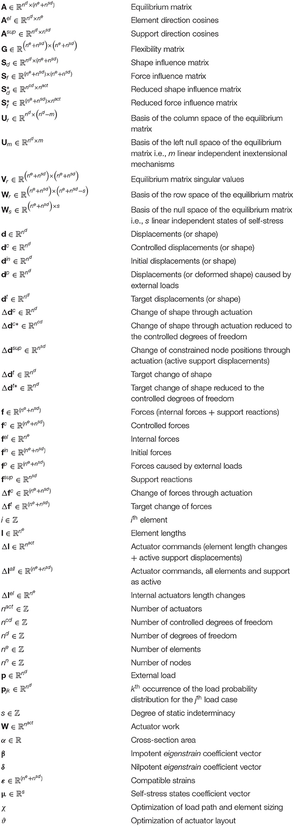
Keywords: adaptive structures, shape control, force control, eigenstrain, force method
Citation: Senatore G and Reksowardojo AP (2020) Force and Shape Control Strategies for Minimum Energy Adaptive Structures. Front. Built Environ. 6:105. doi: 10.3389/fbuil.2020.00105
Received: 27 March 2020; Accepted: 04 June 2020;
Published: 22 July 2020.
Edited by:
Nikos D. Lagaros, National Technical University of Athens, GreeceReviewed by:
Marios C. Phocas, University of Cyprus, CyprusCopyright © 2020 Senatore and Reksowardojo. This is an open-access article distributed under the terms of the Creative Commons Attribution License (CC BY). The use, distribution or reproduction in other forums is permitted, provided the original author(s) and the copyright owner(s) are credited and that the original publication in this journal is cited, in accordance with accepted academic practice. No use, distribution or reproduction is permitted which does not comply with these terms.
*Correspondence: Gennaro Senatore, Z2VubmFyby5zZW5hdG9yZUBlcGZsLmNo; Arka P. Reksowardojo, YXJrYS5yZWtzb3dhcmRvam9AZXBmbC5jaA==
Disclaimer: All claims expressed in this article are solely those of the authors and do not necessarily represent those of their affiliated organizations, or those of the publisher, the editors and the reviewers. Any product that may be evaluated in this article or claim that may be made by its manufacturer is not guaranteed or endorsed by the publisher.
Research integrity at Frontiers
Learn more about the work of our research integrity team to safeguard the quality of each article we publish.