 Adel Francis
94% of researchers rate our articles as excellent or good
Learn more about the work of our research integrity team to safeguard the quality of each article we publish.
Find out more
ORIGINAL RESEARCH article
Front. Built Environ. , 02 April 2019
Sec. Construction Management
Volume 5 - 2019 | https://doi.org/10.3389/fbuil.2019.00036
This article is part of the Research Topic Systems for Construction Management View all 6 articles
The arrival of building information modeling and four-dimensional (4D) simulation is forcing the construction industry to adapt its contractual, operational, and technical modes. Currently, the 4D simulation model is either a bar chart or a linear diagram. Both methods are unsuitable for modeling building projects, as showing the work sequence, circulation, and supply flow between sites is difficult. Spatiotemporal planning is more suitable as a scheduling model, as it considers activities, resources, and spaces simultaneously. However, most of the optimization process based on space planning uses deterministic or stochastic optimization techniques, and these techniques are not viable enough to apply to building construction schedules. The number of parameters is too important for one to consider using algorithmic optimization only. Therefore, this paper proposes a hybrid solution based on spatiotemporal techniques that combine graphical, procedural, and algorithmic aspects. The integration of spaces and operations ensures the continuity of use of spaces and teams, as well as linear production. An approach that prioritizes the critical space on the critical path of activities is proposed.
The fourth industrial revolution with the arrival of building information modeling (BIM) technologies and lean construction methods, including the last planner (Ballard, 2000), the space planning and the Takt time (Frandson et al., 2013), are forcing the construction industry to adapt its contractual, operational, and technical modes.
During the realization phase, 4D modeling techniques can be used to simulate the construction process and thus detect operation succession errors and space use conflicts. Currently, the 4D simulation uses a schedule that model either a Gantt/Precedence diagram or a linear diagram.
The Gantt/Precedence diagram is a timeline scheduling method that combines a graphical representation of the bar chart diagram with precedence dependencies logic. This diagram focuses on defining activities on the time scale and constraints and allocating resources. As it proposes only external constraints and simulates work production through lags, precedence logic lacks precision, diminishing the reliability of the schedule and impairing internal monitoring of activity interdependencies (Francis, 2017). In addition, the calculation of the critical path is based only on time, which compromises its accuracy. Spaces being overlooked, the planner may accidentally schedule many simultaneous activities in the same place. Spaces may also remain underutilized. Then, sites could become congested or relaxed, negatively affecting the project's duration. To plan activities in different work areas, one needs to include the zones in the WBS, which will significantly increase the number of project activities. Adding to this that each activity is plotted on a single row, the graphics rendering becomes complex. Fisk and Reynolds (2014) discussed the visual complexity associated with this method. They reported difficulty reading the dependency lines, which are often extremely close together and cross over other activities, making them confusing to follow without a magnifying glass and a colored pencil to trace the lines. This is why it is hard to follow the logic graphically, to represent the time-space constraints and to optimize the schedule using a Gantt/Precedence diagram.
Resources are allocated to activities; to optimize the process, most research focuses on the best way of leveling these resources without worrying about the linearity of use for the same team and between successive teams. It should be noted that it is quite difficult to ensure linearity using only this planning process, which requires planning activities and then assigning resources. The opposite case is true in planning work for the teams by assigning them activities. The spatiotemporal method proposed in this paper combines three linearities: resources, spaces and activities. By modeling spaces, it is also easier to plan traffic and intermediate stocks.
Linear diagram methods partially solve these shortcomings by ensuring the linearity of resources for the same team and between successive teams. Linear diagrams are initially designed to plan linear projects. Infrastructure projects are good examples; the equipment produces work in a linear and continuous way (e.g., graders, dozers, compactors, scrapers, and sometimes excavators and loaders). Generally, for this type of project, the total number of linear activities is quite small and the quantities executed by type of activity are quite large. All these factors make this diagram well-suited to this type of project.
However, in planning building construction projects, linear diagrams are less suitable. In this type of project, the number of activities is generally important. Even for the same specialty, the variations between jobs make each activity unique. Activities also have to be planned in different areas. Although it is easy to show the linearity of activities in the same area, the multiplication of tasks and zones makes it difficult to show the sequence of work, circulation and supply flow between different zones on a construction project (Francis and Morin-Pepin, 2017).
Repetitive models are more adapted to scheduling building projects. For these projects, repeated tasks are assigned from unit to unit or from floor to floor. This differentiates them from linear projects in which machinery is operating continuously. We can distinguish two types of repetitive projects: (a) vertical projects, such as multi-story buildings and (b) horizontal projects, such as the construction of several similar units. In repetitive vertical projects, some activities are non-repetitive activities, such as the foundation and the roof, while others are repeated from one floor to another, such as structure, architectural finishing, and services. In repetitive horizontal projects, most activities are repetitive, and the work of several units can be planned simultaneously to accelerate the project schedule. The number of specialty teams can be calculated with the quotient of the duration required to complete a single unit by the total time available to complete the work of this specialty for all units (Francis, 2015).
Combining repetitive modeling to space planning methods are therefore more suitable. The objective of the space planning is to link the spatial and temporal aspects, promote efficient use of the site, define optimal site occupancy rates, and ensures suitable rotation of the workforce in the different spaces. Space planning considers, in addition to activities and resources, the areas of the site involved in the planning of a project. Indeed, it is important to consider spaces. Unlike manufacturing work, where the work comes to the workers, on a construction site, the labor moves to work (Ballard and Howell, 1998). Workspaces are often neglected in construction site planning methods, which causes congestion or conflict (Chua et al., 2010).
The optimization of construction schedules for building projects based on space planning generally uses deterministic or stochastic optimization techniques. Some have used statistical methods to manage site occupancy (Rodriguez-Ramos, 1982; Tommelein, 1989; Yeh, 1995). However, these methods ignore the possible reuse of the site space. Others use dynamic site optimization techniques (Zouein and Tommelein, 1999; Xu and Li, 2012; Kumar and Cheng, 2015; Farmakis and Chassiakos, 2018) by using interactive selection, computer-based positioning of resources or dynamic facility relocation from phase to phase. These purely algorithmic solutions are excellent for advancing scientific research. On the other hand, these methods are not too adapted to be used for the optimization and follow-up of schedules on building sites. Building sites are very complex, and the number of parameters is important to consider during modeling. Considering all parameters makes the model very intricate and time-consuming. The cost of modeling will also be disproportionate compared to the benefits. Thus, each model selects the parameters believed to be important and neglects all others, and neglecting parameters will have negative impacts on the results. In addition, some parameters depend on site circumstances or management decisions; e.g., delays in approvals or delivery of materials, labor absences, modifications, and weather conditions. In these cases, this paper supports that nothing supersedes the decisions of those involved in the execution work on-site.
This paper supports the idea that graphical solutions combined to the last planner system are more suited to this type of optimization and can be considered decision support systems. Law (2015) cites that the estimation of simulation parameters is a key problem in construction simulation, especially for near-future schedule prediction in the construction phase. Because simulation is a computer-based statistical sampling experiment, the sampling basis, i.e., the density of simulation parameters, directly influences the simulation accuracy.
Few studies have addressed the optimization of building construction schedules based on graphical approaches. Some propose defining spaces according to their occupation statuses (free, occupied) (Winch and North, 2006), and others according to their types of use (work, storage, circulation) (Riley, 1994; Riley and Sanvido, 1995) or according to the needs of stakeholders (Frandson and Tommelein, 2014). Models have also described the behavior of spaces according to the nature of the work performed there (Riley and Sanvido, 1997) or according to their physical evolutions during the activity implementation process (Zouein and Tommelein, 2001).
Frandson and Tommelein (2014) developed Takt time planning. Takt planning splits the project into zones that allow for linear Takt time and the continuity of work. Francis (Francis, 2004, 2013, 2016) developed the Chronographical concept for modeling project information. This concept allows for alternating from one visual approach to another via the manipulation of parameters. The spatiotemporal model (Francis and Morin-Pepin, 2017) demonstrates construction operations on the foreground and site spaces in the background. The model also considers various execution constraints, including space management and traffic. This method enables the visual management of the project's progress and space conflicts.
Chronographic modeling is based on visual graphical approaches, including spatiotemporal approaches, which facilitates the sharing of information and the graphic optimization of schedules. Chronographic modeling focuses on the communication of information with the possibility of alternating from one visual approach to another via the manipulation of graphic parameters. This allows for the grouping, prioritization and classification of project information. Its advantage over existing solutions for 4D simulation is that it integrates space planning into the schedule. The concept is based primarily on critical space rather than on a critical path of activities.
The conceptual framework of the Chronographic standard protocol (Francis, 2016) defines the graphical protocol for physical (production) entities, their properties and logical constraints, which determine the relationships between these entities and the execution process. Physical entities can be arranged graphically using various organizational means of distinction, association, scales, and attributes. Activities can be plotted in parallel and in series. Activities can have one or more internal divisions. These divisions can be related to external or internal scales. The external scales usually represent the time, while the internal scale usually represents the quantities. Internal divisions extend the relationships between the activities to point-to-point relations, generating realistic dependencies and new types of floats (Francis and Miresco, 2006).
The conceptual framework also defines the organization model and the representation approaches of these entities. The project schedule can be modeled through tabular and graphical means, namely: (i) tables that show detailed information about an element (e.g., activity start date and duration); (ii) cross-tabulations that present analytical interrelations between physical entities; (iii) pure logic networks; (iv) time-scaled diagrams and networks; (v) Chronographic modeling; (vi) 4D models; and (vii) charts.
The result is the presentation of the same project schedule through various compatible approaches. The planner can alternate from one approach to another through the manipulation of graphics parameters. Visual communication is then improved through layering, sheeting, juxtaposition, alterations, and permutations, allowing for groupings, hierarchies and the classifying of project information. In this way, graphic representation becomes a living, transformable image. The comprehensive results can be found in Francis (2013, 2016).
The Chronographic method identified five (5) major successive stages of the implementation of the construction phase of a building project, namely the creation of spaces (e.g., addition of new floors); the systems (e.g., ventilation ducts); the division of spaces (e.g., partitions); the finishing (e.g., painting); and the closing of spaces (e.g., carpet laying). The Chronographic method graphically models these stages by creating five levels of graphical layers. Each is subdivided into zones according to the stage of construction, creating a dynamic hierarchy of spaces. Figure 1A shows the five layers and their division into zones. Each zone is identified by a different identification (ID) and color (and/or texture). At each of these five stages, the layout of the construction site changes its configuration. New spaces will be added, creating new work areas. Other spaces will be fenced or closed, thus limiting the movement of people, materials and the reverse cycle and at the same time making the management of sites more complex.
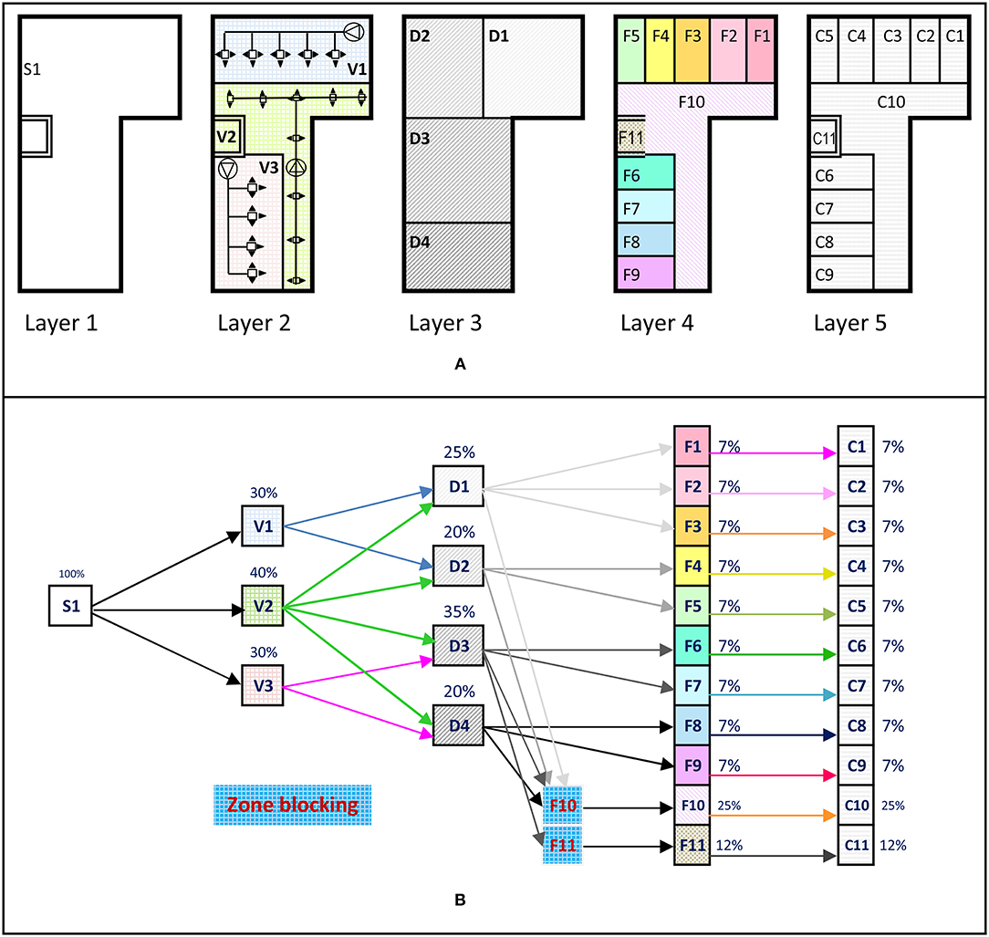
Figure 1. Weight and hierarchy of layers and zones of the site according to Chronographic modeling. (A) Modeling of layers and zones, (B) hierarchy of layers and zones.
Each of the site's operations belongs to one of these stages. Thus, pouring concrete for a new floor slab will create new workspaces. The systems will be installed by sector or by system. The partitions will cut the spaces to create smaller areas for finishing work. Finally, to avoid damaging the floor finishes, the manager will close areas to constrain the movement of people and materials. For this, the ease of circulation and stock on the floors will depend on the stage of construction. For example, after the installation of the divisions, circulation, and stock will be more complex and will require more coordination.
The lower part (Figure 1B) establishes the hierarchy of layers and zones and the weight of each zone with respect to its layer. The hierarchy creates a network of a succession of the zones according to the order of execution on the building site. Each zone is thus linked with other zones on the predecessor and successor layers. This non-time scaled scheduling network is based on work locations and location breakdown structure (LBS) instead of activities such as traditional critical path method (CPM) networks. If durations are added to the zones, the critical path of the zones can be obtained. Figure 5 shows the succession of these spaces in the background of the figure, and Figure 6 shows the same network of spaces but using time-scaled modeling.
With this system, operations on a zone of a certain layer can start only when all of the predecessor layers that interfere with it are released. For example, zone D2 of the third layer (division of space) is released only when all of the operations on zones V1 and V2 of the second layer (system) are completed. In addition, to ensure circulation on the floors, some areas must be blocked, delaying operations for a period. These blocked areas are added to the space hierarchy. For example, the elevator shaft (zone F11) is blocked for vertical circulation between the floors of the building. This blocking delays the installation of the elevator until the release of this blockage. Another example concerns the corridor (zone F10), which has been blocked for a certain period during the finishing phase to facilitate horizontal circulation. This blocking delays the finishing work of the corridor.
The main goal of this research is to model and optimize the site operation and execution process for construction buildings projects based the Chronographic modeling. The aim is to link spatial and temporal aspects, promote efficient use of the site, define optimal site occupancy and ensure suitable rotation of the workforce in different spaces.
The principal strength of the proposed method is its relative ability to facilitate the modeling and optimization of site operation using simple graphical means. This paper contributes to the existing body of knowledge by extending the optimization process from purely algorithmic solutions to a hybrid process based on graphical, procedural, and algorithmic techniques.
The main objective of this research is the optimization of building construction schedules based on graphical, procedural, and algorithmic techniques. This hybrid spatiotemporal approach combines the optimization of the use of construction site spaces and execution teams. It promotes the continuity of the use of spaces by maximizing a site's occupancy rate. It also ensures the continuity of work through linear production for the same team and parallel linearity between the various successor teams.
This research is limited to building construction projects. The suggested optimization system will yield better results in the case of multi-story buildings (e.g., towers), the case of several similar buildings, the case of a large-scale building in which work is repeated between different zones, or for a combination thereof. For other types of buildings, mathematical optimization must be limited, and the contribution of the manager should be increased.
It should be noted that the duration of a project based on this approach depends primarily on the optimal use of the construction site by ensuring the best occupancy rate—and not just on the critical path of the activities. We therefore prioritize the critical space on the critical path. The reason for this is that a relaxed and underused site unnecessarily delays the schedule. Conversely, an over-occupied site increases space and interpersonal conflicts. Thus, the method involves creating the project schedule based on the succession of critical spaces occupied by operations, circulation or intermediate stock.
The method also considers non-productive activities as intermediate stocks, garbage, recycling materials, temporary installations and on-floor traffic. These non-productive activities occupy space and limit or delay on-site operations. If these delays increase the total project duration, they will also increase the indirect costs and must therefore appear on the critical space's path. They are thus considered to be wastes and must be reduced as much as possible. An extensive study of traffic, temporary installations, daily cleaning and pull or just-in-time supply strategies must therefore be considered in the optimization approach.
It is completely clear that many modeling constraints must be considered. First, there are the constraints of the succession of activities. Second, we must consider the resource constraints, especially with the multiplication of stakeholders and knowing that the majority of the work is performed by subcontractors. Third, there are space constraints on the site with all of the occupation conflicts it can generate. Finally, there is the variability in the execution conditions, the unforeseen and unexpected changes. Thus, the quantity of the parameters to be modeled is important. Any parameter not considered will negatively affect the optimization result. For this reason, it is practically impossible to proceed with a purely mathematical optimization. Graphical or hybrid optimization approaches involving the manager and other stakeholders are more realistic.
The management of space and occupancy rates is done by period and by involving the real people implicated in the project. Based on the last planner and the Takt planning techniques, the model requires less effort to build and monitor than the traditional methods. These approaches provide realistic results with fewer errors. The proposed system therefore favors the manager's decision-making and is considered to be a decision support system.
To facilitate the exposure and understanding of the proposed optimization process, this paper uses the activities to demonstrate only the succession constraints. The optimization of activity-based deadlines, including time-cost trade-off techniques, has been widely discussed in the literature.
The critical space on the critical path of activities is leveled by relaxing or compressing the project based on the site occupancy rate. This could be achieved by decreasing or increasing the number of teams, which would increase or decrease the number of activities of the same type running in different areas. An example of this is using two teams to install Gyprock plasterboard in two areas to occupy more space while reducing the time in half, or conversely, reducing the number of teams to relax the use of spaces. This logic is completely different from scheduling optimization techniques based on increasing the overlaps between various types of successors' activities. An example of this is placing electrical wires in metal studs before stud installation is completed in one area. This overlap does not increase the number of resources of the same type but causes the successor teams to intervene more quickly. Although it decreases the duration of the project, it increases the risk of errors and therefore the rework.
The project site's occupancy rate calculation is calculated per period as the sum of the production of the occupancy rates and each zone's relative weight. This method attributes a relative weight to each zone that corresponds to its impact on site circulation. For example, a corridor used as the main path for circulating materials has much more weight than a closed room does. Graphically, the occupancy rate is demonstrated by a range of warm-cold colors, with the red color being the hottest and the violet color being the coldest.
The question is, how can the manager define the right occupancy rate for the site? Two scenarios have been proposed in the past. The first based on experience, the manager defines a good level of occupation, for example, 70%. This system also defines the occupation ranges; for example, between 0 and 20%, there is little or no activity on the site, and between 80 and 100%, the site is congested. In the second method (Francis and Morin-Pepin, 2017), the optimal occupancy rate is set to 100%. This method blocks out areas where jobs should not be performed. For example, we close the corridor for a certain period for circulation purposes. Other areas may be blocked for the intermediate storage of materials or job protection. These blocked zones are counted as occupied in the calculation of the occupancy rate. This achieves the optimal rate of 100% use of the site.
Linear methods are designed to ensure the continuity of resource use and to support stable and optimized production. Linear methods are usually convenient for linear infrastructure projects, such as those involving roads and railways, where machinery is operating continuously. This differentiates them from repetitive projects, where assigning tasks are usually repeated from unit to unit or from floor to floor. We can distinguish two types of repetitive projects: vertical projects, such as multi-story buildings, and horizontal projects, such as the construction of several similar buildings units.
In building projects, the linearity of repetitive activities is just as important. This linearity must allow for the continuity of the use of resources and spaces. All resources for repetitive activities are planned in a continuous way. Linearity means that a team works continuously and progresses from one zone to another without stopping. The teams that succeed each other progress on the site at the same pace. This means that as soon as a team frees a zone, the next team occupies the liberated zone. It also means that there is a continuity of the use of the spaces and that the occupancy rate of the site is stable.
Figure 2 shows the planning of a five-story building in which five activities are carried out: stud installation, Gyprock installation, painting, suspended ceiling installation, and flooring. Each floor is considered to be a single work area except for the two painting and suspended ceiling activities, for which each floor is divided into two zones (Z1 and Z2). This figure models the project under different approaches, line chart (Figures 2A2,B2) and the Gantt chart (the four other figures). In addition, in Figures 2A1,A2,A3, the activities are grouped by floor, whereas in Figures 2B1,B2,B3, floor (F1 to F5) and zones (Z1 and Z2) are grouped by Work Breakdown Structure WBS.
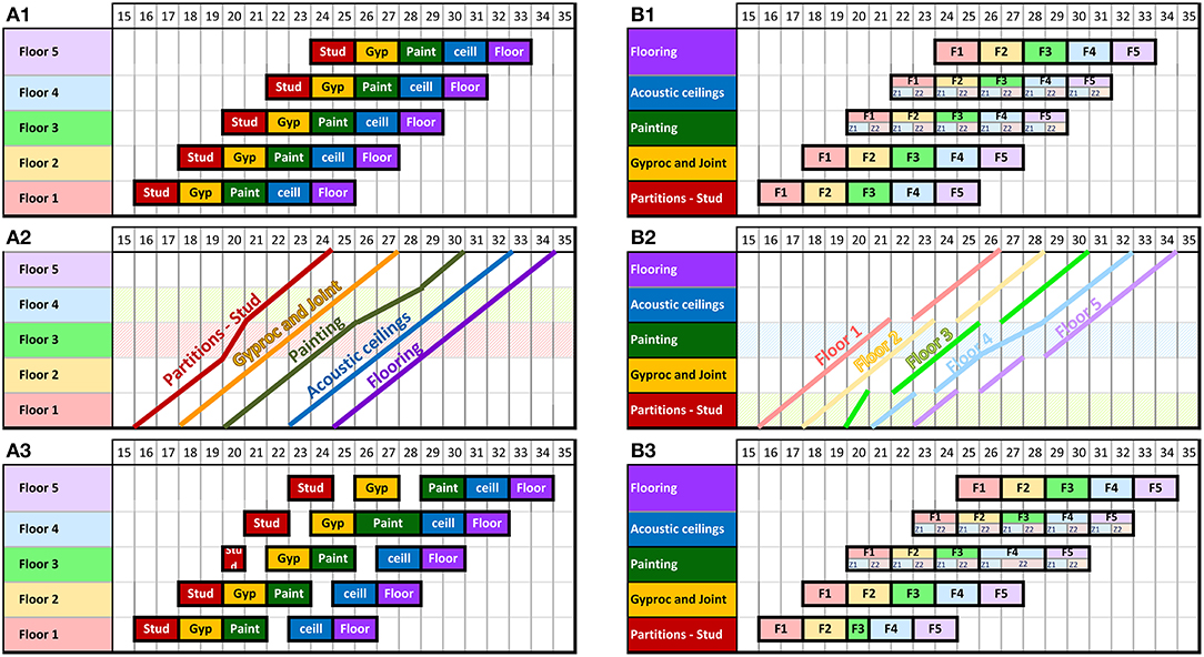
Figure 2. Linearity and Takt time planning. (A1) Gantt chart grouped by floor and with uniform production; (A2) line chart grouped by floor; (A3) Gantt chart grouped by floor; (B1) Gantt chart grouped by WBS and with uniform production; (B2) line chart grouped by WBS; (B3) Gantt chart grouped by WBS.
In Figures 2A1,A2,B1,B2, the execution is linear. The zones are divided so that the amount of work in each of them is almost equivalent. The number of teams (or people) in each specialty is adjusted so that the duration per floor or per zone is the same. We vary the productivity to fix the duration. Thus, all activities have the same duration per zone (2 days each). The rotation of a team on different floors or zones is therefore linear. This execution process is called Takt time planning. Takt time planning defines the frequency of team rotation between zones to stabilize work on building sites [23].
In Figures 2A3,B3, perfect linearity could not be maintained. To ensure Takt time planning, the Chronographic method sets the free float value equal to zero between the Takt activities. This imposition delays the start of predecessor activities to bind them with their successors. The delayed start is called the “Takt start.” The “Stud” activity of floor 3 can be performed in 1 day, and the “Paint” activity on the fourth floor should be longer with a duration of 3 days. The delay caused by the “Paint” activity on floor 4 delays the “Ceill” activity, which has to start early on the 29th day. To ensure the Takt process, the start of the “Ceill” activity on floors 1 to 3 is also delayed when their free float value is set to zero. Thus, the Takt start of these activities is later than their early start, creating start free floats, which are calculated by the differences between their Takt start and their early start. In this case, the manager has to choose between the continuity of the use of crews and the continuity of using the working areas. In Figure 2B3, the decision is to ensure the optimal use of resources with team continuity.
The objective of graphic optimization is to ensure the continuity of the use of resources and spaces. The study of linearity in the evolution of activities makes it possible to evaluate this continuity. Four cases arise:
1) The lines diverge; this means that the space between the lines (Figure 3A) and therefore the start free floats increases. In this case, linearity can be adjusted by relaxing the productivity of predecessor activities (by decreasing the number of teams) or by accelerating the production rate of successor activities (by increasing the number of teams). The decision could be made according to the availability of the teams;
2) The lines converge; this means that the space between the lines (Figure 3B) and therefore the start free floats decreases (Figure 3B). In this case, the linearity is adjusted by accelerating the production rate of the predecessor activities or by relaxing the productivity of the successor activities;
3) A relatively parallel linearity (Figure 3C) means a good succession of work. Start free floats also remain constant. This does not mean that the occupation of the site is optimized. For the purpose of optimization, the number of teams is adjusted to ensure the optimal occupancy rate of the spaces of the project site;
4) Finally, two crossing lines usually mean a logical error unless the predecessor and successor activities can run in parallel.
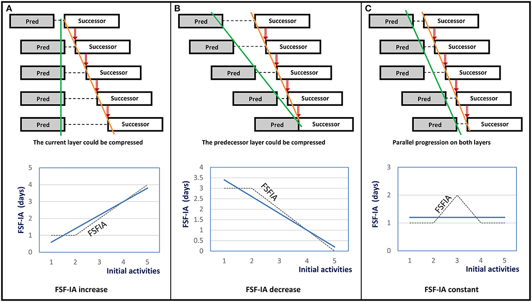
Figure 3. Trend line of the free start float for initial activities (FSF-IA). (A) FSF-IA increase. (B) FSF-IA decrease. (C) FSF-IA constant.
According to the graphical optimization process proposed by the Chronographic method, the optimizations are done by layer. To do this, one must first define the initial and terminal activities of a layer. An activity that has no technical predecessor in the same layer is considered to be an initial activity of the layer, and an end that has no technical successor in the same layer is considered to be a final activity of the layer. The same layer can have several initial and final activities.
In Figure 3, if the predecessor activities, colored gray, are on the previous layer, the successor activities become initial activities. To optimize a layer, it is first necessary to calculate the initial free floats of all of the initial activities. These floats are called “free start float for initial activities” (FSF-IA). If the curve drawn for these margins is not linear, we trace the linear trend line (blue bold line on Figure 3). If the trend line is ascending, which means that the FSF-IA generally increase, the optimization is done in the same layer. If the trend line is descendant, which means that the FSF-IA generally decrease, we must go back to optimizing the previous layer. Finally, if the trend line is horizontal, which means that the FSF-IA are relatively equivalent, we decrease the FSF-IA value to the maximum.
Thus, the optimization process is based on the linearity with parallel progress rates between the successor teams. It is also based on maximizing the occupancy rate of the site. The optimal occupancy rates are set to 100%. This is possible without cluttering the site because the method blocks out areas where jobs should not be performed, as for circulation, for storage and for the protection of works.
The role of the manager is to coordinate the succession of the subcontractors' works between the zones and to occupy the site in an optimal way. He will define, in collaboration with the subcontractors, the duration of each activity by zone and the number of necessary teams. The division of the zones is done with the objective of continuity in the site operations and occupation. Good planning assures the linearity of repetitive activities. This linearity is ensured by the addition of resource links between repetitive activities. The method recommends not adding resource links for non-repetitive or one-off activities and uses only technical links.
The level of detail of the schedule depends on the level of control. It must not in any case exceed the level of authority of the manager. For example, it is useless for the general contractor's manager to plan the sub-activities and resources of the subcontractors. It is also advisable to limit the level of detail to the maximum. A schedule with high detail will hinder good planning and optimization, as the manager will lose the overall view of the schedule and focus on the details. These details may be in the form of sub-tasks, activity completion steps or a list of jobs to be done (not shown on the modeling view).
In order to prepare the project schedule, the manager begins spatiotemporal modeling. Figure 4 shows the Chronographic planning process.
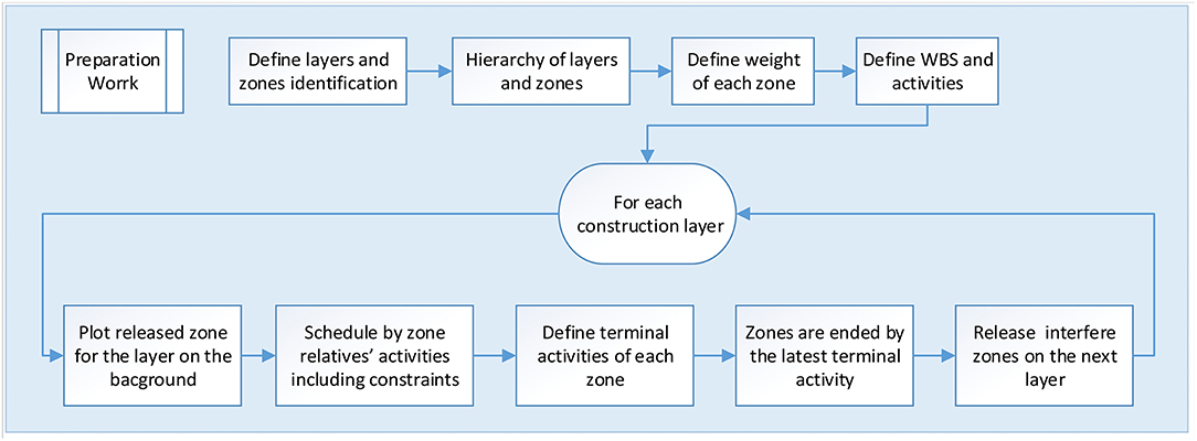
Figure 4. Spatiotemporal Chronographic planning process.
The example shown in Figure 5 details these steps by modeling the schedule of the building floor shown in Figure 1. In this modeling, the scheduler defines five levels of layers for space management, namely: (i) the creation of spaces for structure erection (zone S1); (ii) the systems (zones V1 to V2); (iii) the division of spaces for partitions, electrical wiring and plumbing pipes (zones D1 to D4); (iv) the finishing (zones F1 to F11); and (v) the closing of spaces (zones C1 to C11). Zones are identified by different IDs, colors, and/or textures.
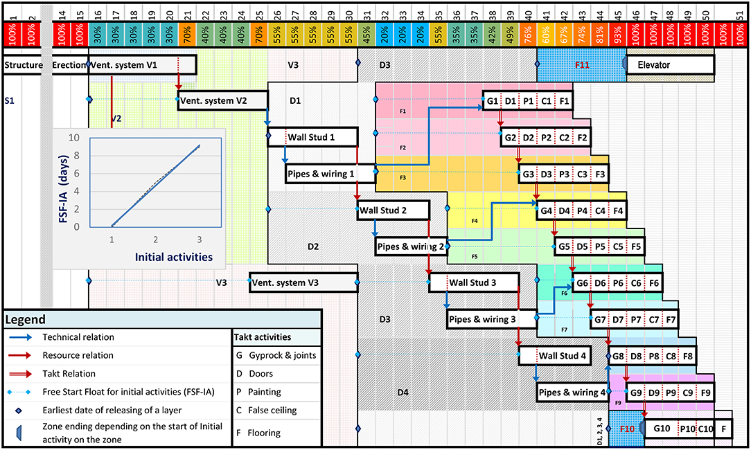
Figure 5. Spatiotemporal Chronographic planning of a building floor.
The approach uses graphical modeling showing construction operations in the foreground and site spaces in the background (see Figure 5). It uses colors and attributes in accordance with the Chronographic protocol (Francis, 2016).
After this preparatory work, the manager begins spatiotemporal modeling. The modeling steps are detailed below:
1. First layer: this layer is composed of a single zone (S1) demonstrated in the background of the figure. To simplify the model, the structure erection is demonstrated in a single activity without any detail. After this activity is completed, this layer ends and releases the subsequent layer;
2. Second layer: the three zones of this layer (V1 to V3) are released and modeled in the background. Activities are planned in the foreground. This layer has three initial activities (ventilation system). The subcontractor has decided to put a single team for the installation of the three systems successively. Resource links (red lines) between activities are therefore necessary;
3. Third layer: after the work of each zone of the second layer is completed, the zones that interfere with them on the third layer are released. The four zones (D1 to D4) depend on zone V2. In addition, D1 and D2 depend on V1 and D3, and D4 depends on V3. These zones are modeled in the background, and the initial activities (“Wall Stud”) can start. Because there is only one team, resource links, shown with red lines, are added between these four activities. Technical constraints are also added for their successor activities (“Pipes and Wiring”);
4. Fourth layer: The manager must proceed in the same way as with the previous layer. The main difference is that the links between the activities of the same types (e.g., G1 to G9) are Takt links (red double line). This means that there must be zero free floats between them. Because activity G8 is delayed by zone D4, the starts of activities G1 to G7 are also delayed. Delayed starts are called “Takt starts.” This layer also contains two blocking zones (F10 and F11). These blocking areas are usually reserved for traffic or storage. A blocking zone may have a flexible duration. This means that its end depends on the start date of the successor activity. To make a zone flexible, its end is controlled by the “zone ending depending on the start of the successor activity” entity. In addition, if this successor activity is an initial activity, its FSF-IA will be zero (see Figure 5);
5. Fifth layer: this layer is a zone closure layer. This means that it does not contain any activity, and the zones are simply blocked. Their graphical modeling is important for calculating the occupancy rate of the site.
Figure 6 shows the time-scaled scheduling network of zones according to the execution process on the building site. Each zone is linked with its predecessor and successor zones. This network is based on work locations instead of activities, such as traditional CPM networks. By adding the zones' occupancy durations, we obtain the critical path (S1, V3, D4, F9, and F10) framed in red as shown in the figure.
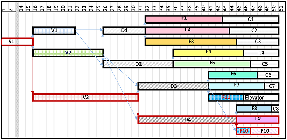
Figure 6. Time-scaled scheduling network of zones.
In the same way, the network of zones, like the network of activities, provides only partial information. The optimization of these networks is therefore more complex, and the result is questionable due to the lack of information on activities and resources in the case of the zones' network, and on areas and resources in the case of the activities' network. Spatiotemporal modeling is more suitable for planning, coordinating, monitoring, and optimizing construction schedules.
The spatiotemporal optimization process optimizes the use of both spaces and teams. This hybrid process is based on graphical, procedural and algorithmic techniques. It integrates the manager into the decisions. Figure 7 summarize the optimization process.
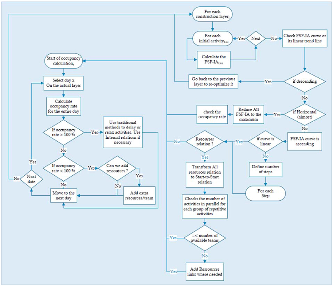
Figure 7. Spatiotemporal Chronographic optimization process.
The detailed process is as follows:
1. The optimization is done by layer in order. The process optimizes the first layer and then proceeds to the next layer, and so on. The process starts by optimizing the first layer of the creation of spaces for the steel structure erection (Figure 8). In this case, there is no place for optimization. Then, the planner should move to optimize the second layer, and so on.
2. As soon as all the final activities on a certain zone of a predecessor layer are completed, the zones of the successor layer that interfere with it are released according to the hierarchy shown in Figure 1. The initial activities of these layers zones could start.
3. At the beginning of each layer, it is necessary to check the FSF-IA curve or its linear trend line if it exists. If the curve is ascending, which means that the FSF-IA generally increase, the optimization is done on the same layer (see the next point, point 4). If the curve is downward, which means that the FSF-IA generally decrease, the process has to re-optimize the previous layer (see point 5). Finally, if the curve is horizontal, which means that the FSF-IA are relatively equivalent, the process sets the FSF-IA to zero (see point 6).
4. If the curve or the linear trend line is generally descending, the manager must go back to the previous layer to re-optimize it. Thus, the optimization process uses a forward/backward process of compression or relaxation according to the occupancy rates. In the previous layer, the same optimization process described in the previous section is used.
5. If the curve or linear trend line is generally horizontal, the FSF-IA are reduced to the maximum. Then, we check the occupancy rate per period. If this rate is low, it means that the site is relaxed. The process proposes going back to the previous layer to optimize it. The manager must work with the subcontractors to increase the number of teams. If impossible, he will move to the next layer.
6. If the curve or the linear trend line is ascending, the optimization is done in the same layer. Two cases may arise:
a) If the curve is linear: For the current layer, it is necessary to transform all of the resources' relations to start-to-start relations. Recall that resource links are used only between repetitive activities. After this transformation, the system checks the number of activities in parallel for each group of repetitive activities. For example, in the third layer (Figure 8) for each of the repetitive activities of “Wall Stud” and “Pipes and Wiring,” the number of activities in parallel is four. A maximum of four teams of each type can be planned. The system should show to the manager the number of required teams and the minimum, optimal and maximum number of teams for each repetitive group. The system must also demonstrate the number of available teams for each repetitive group. For example, if there are four teams for the “Wall Stud” activity and two teams for the “Pipes and Wiring” activity, the manager will usually have to take the smallest number of teams available. There is no point in taking four “Wall Stud” teams because in any case, workers cannot close the walls sooner, knowing that only two “Pipes and Wiring” teams are available. It is not necessary to remember that in the opposite case, it is impossible to have two teams for “Wall Stud” and four teams for “Pipes and Wiring.” The manager can adjust the system so that this step is done automatically. The decision will therefore be to have the smallest number of teams available for all repetitive successor activities. Finally, if the number of chosen teams is smaller than the number of successor activities in parallel, resource relationships will be added.
b) If the curve is not linear and a linear trend line is drawn, we must proceed in the same way as with the previous point (4a), with the exception being that the optimization process will be done by steps. For example, in Figure 8, the calculation of FSF-IA (see Table 1) shows that there is no increase between the G4 and G5 activities. The FSF-IA in both cases is equal to 3 days. It also shows that the two layers of F4 and F5 do not begin at the same time. First, we eliminate the resource links between G1 and G4 activities. Then, we study the offset between the beginning of the layers (in this case, it is F5 and F4). If this offset is equal to or greater than the duration of the repetitive activities, there will be no overlap. We can also eliminate all of the resource links of this second step except for the first one (in our case, between G4 and G5), and then, we move on to the next step.
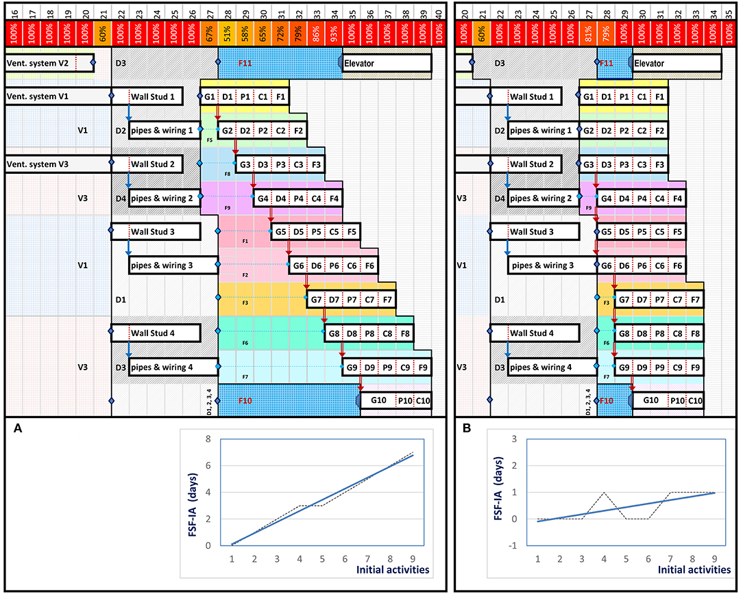
Figure 8. Choice number 1 for the scheduling optimization. (A) Optimization of third layer. (B) Optimization of the fourth layer.
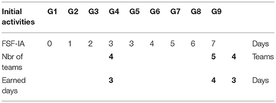
Table 1. The calculation of FSF-IA and number of teams.
If repetitive activities are Takt activities, it is mandatory to have the smallest number of teams for all groups. Because the free margins are zero, the beginning of the predecessor activities is delayed in all cases.
With such a planning and optimization process, the occupancy rate cannot exceed 100%. In addition, no conflict or clutter is expected. The manager or system will check the occupancy rate per period. If this rate is low, this means that the site is relaxed. He must therefore see with the subcontractors how to increase the number of teams.
The system will calculate the maximum number of teams, the gain in days and the percentage for each choice of the number of teams. The system will also be able to calculate the additional cost of adding teams and the gain on indirect costs for the time saved. This will allow the manager to make an informed decision. The manager could also decide to launch simulations of the optimization process based on time-cost trade-off techniques based on techniques already known and widely treated in the literature.
The two figures of 6 and 7 demonstrate the impact of the optimization choices on the schedule and occupancy rate.
In Figure 8, after the second layer is released, the linear trend line is ascending (see curve in Figure 5). Optimization is done in the same layer. The resource links are removed, and the schedule shows that we work in the same time (V1 to V3) at the same time. The manager has accepted this choice and has planned three teams.
Because all of the areas of the third layer depend on the V2 zone, they are completed, and the third layer is released. The initial Wall Stud activities can start. The linear trend line is ascending; the optimization is done in the same layer. The resource links are removed, and the timeline shows that we can all run. Because four teams of each type of activity, “Wall Stud” and the “Pipes and Wiring,” are available, the manager can accept this choice and use four teams.
For the fourth layer, the linear trend line is also ascending. The curve shows that the process will be applied in steps because there is no increase between activities G4 and G5. The FSF-IA in both cases are equal to 3 days. It also shows that the two layers of F4 and F5 do not begin at the same time. Firstly, we eliminate the resource links between G1 and G4 activities. Then we study the offset between the beginning of the layers (in this case it is F5 and F4). Because the offset is equal to the duration of the repetitive activities, there will be no overlap; we will also eliminate all of the resource links of this second step except for the first one (in our case, between G4 and G5). The maximum number of teams is four for the first step and five for the second step. The manager decides, perhaps due to the availability of teams or based on a time-cost trade-off analysis, to engage only three teams for each of the Takt activities (G, D, P, C, and F).
The same optimization process used in Figure 8 is applied in Figure 9; however, the choices are different. In the second and the third layer, the manager always chooses to have a single team (Figure 9A). Thus, for the fourth layer, the linear trend line is generally descendant. If the planner wants to compress this layer, he should use the backward process and try to re-optimize the previous layer by engaging at least two teams for the “Wall Studs” and “Wiring and Pipes” activities (Figure 9B). The rest of the process therefore becomes identical to that of Figure 8.
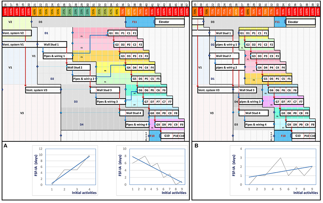
Figure 9. Choice number 2 for the scheduling optimization. (A) Optimization of third layer. (B) Optimization of the fourth layer.
In conclusion, the integration of spaces, operations and temporal aspects promotes efficient use of building sites and helps managers maximize the site occupancy rates, ensure suitable rotation of the workforce between zones and support linear productions of spaces and teams. The proposed hybrid optimization (based on spatiotemporal techniques) combines graphical, procedural and algorithmic aspects and proves to be a better solution for building construction sites. This approach prioritizes the critical space in the critical path of activities by defining the optimal site occupancy rates.
The proposed system also promotes managerial decision-making; it is therefore deemed a decision support system. Purely algorithmic optimizations are hard to implement for building sites due their complexity and the number of parameters to be considered during the optimization process. In that case, this paper supports the concept that nothing supersedes the decisions of those involved in the execution work on-site.
This research is limited to the modeling and optimization of building construction projects. The suggested optimization system will yield better results in the case of multi-story buildings, several similar buildings, large-scale buildings in which work is repeated between different zones or a combination thereof. Future works will extend the process to other types of projects and will automate the links between the proposed spatiotemporal schedules with 3D models to create a 4D spatiotemporal simulations.
All datasets generated for this study are included in the manuscript and/or the supplementary files.
The author confirms being the sole contributor of this work and has approved it for publication.
The author declares that the research was conducted in the absence of any commercial or financial relationships that could be construed as a potential conflict of interest.
Ballard, G. (2000). The Last Planner System of Production Control. PhD. thesis, Department of Civil Engineering, University of Birmingham, Birmingham.
Ballard, G., and Howell, G. (1998). Shielding production: essential step in production control. J. Constr. Eng. Manag. ASCE 124, 11–17. doi: 10.1061/(ASCE)0733-9364(1998)124:1(11)
Chua, D. K. H., Yeoh, K. W., and Song, Y. (2010). Quantification of spatial temporal congestion in four-dimensional computer-aided design. J. Constr. Eng. Manage. 136, 641–649. doi: 10.1061/(ASCE)CO.1943-7862.0000166
Farmakis, P. M., and Chassiakos, A. P. (2018). Genetic algorithm optimization for dynamic construction site layout planning. Org. Technol. Manag. Constr. 10, 1655–1664. doi: 10.1515/otmcj-2016-0026
Fisk, R. E., and Reynolds, W. D. (2014). Construction Project Administration, 10th Edn. Franklin Lakes, NJ: Pearson Education Inc.
Francis, A. (2004). La Méthode Chronographique Pour la Planification des Projets de Construction. Ph.D. thesis, École de technologie supérieure, University of Quebec, Montreal. Avaliable online at: http://espace.etsmtl.ca/692/ (accessed May 19, 2004). (in French).
Francis, A. (2013). The chronographical approach for construction project modelling. Manag. Proc. Law 166, 188–204. doi: 10.1680/mpal.12.00009
Francis, A. (2015). “Applying the Chronographical approach for modelling to different types of projects,” Proceedings of the 5th International/11th Construction Specialty Conference (ICSC 15), (Vancouver, BC).
Francis, A. (2016). A chronographic protocol for modelling construction projects. Manag. Proc. Law 169, 168–177. doi: 10.1680/jmapl.15.00039
Francis, A. (2017). Simulating uncertainties in construction projects with chronographical scheduling logic. J. Constr. Eng. Manage. 143, 1–14. doi: 10.1061/(ASCE)CO.1943-7862.0001212
Francis, A., and Miresco, E. T. (2006). A chronographic method for construction project planning. Can. J. Civil Eng. 33, 1547–1557. doi: 10.1139/l06-148
Francis, A., and Morin-Pepin, S. (2017). “The concept of float calculation based on the site occupation using the chronographical logic,” Procedia Eng. 196, 690–697. doi: 10.1016/j.proeng.2017.07.235
Frandson, A., Klas, B., and Tommelein, I. D. (2013). “Takt time planning for construction of exterior cladding,” in 21st Annual Conference of the International Group for Lean Construction, (Fortaleza).
Frandson, A., and Tommelein, I. D. (2014). “Development of a takt-time plan: a case study. construction research congress 2014: construction in a global network,” in Proceedings of the 2014 Construction Research Congress, May. (Reston, VA: American Society of Civil Engineers), 1646–1655. doi: 10.1061/9780784413517.168
Kumar, S. S., and Cheng, J. C. (2015). A BIM-based automated site layout-planning framework for congested construction sites. Automat. Constr. 59, 24–37. doi: 10.1016/j.autcon.2015.07.008
Law, A. M. (2015). “Statistical analysis of simulation output data: the practical state of the art,” in Proceedings of the 2015 Winter Simulation Conference, Huntington Beach. doi: 10.1109/WSC.2015.7408297
Riley, D., and Sanvido, V. E. (1995). Patterns of construction-space use in multistory buildings. J. Constr. Eng. Manage. 121, 464–473. doi: 10.1061/(ASCE)0733-9364(1995)121:4(464)
Riley, D., and Sanvido, V. E. (1997). Space planning method for multistory building construction. J. Constr. Eng. Manag. 123, 171–180. doi: 10.1061/(ASCE)0733-9364(1997)123:2(171)
Riley, D. R. (1994). Modeling the space behavior of construction activities. Ph.D. dissertation, Department of Architectural Engineering, Penn State University, University Park, TX.
Rodriguez-Ramos, W. E. (1982). Quantitative Techniques for Construction Site Layout Planning. Ph.D. dissertation, University of Florida, Gainesville, FA.
Tommelein, I. D. (1989). SightPlan - An Expert System that Models and augments human decision-making for designing construction site layouts. Ph.D. dissertation, Department of Civil Engineering, Stanford University, Stanford, California.
Winch, G. M., and North, S. (2006). Critical space analysis. J. Constr. Eng. Manag. 132, 473–481. doi: 10.1061/(ASCE)0733-9364(2006)132:5(473)
Xu, J., and Li, Z. (2012). Multi-objective dynamic construction site layout planning in fuzzy random environment. Automat. Constr. 27, 155–169. doi: 10.1016/j.autcon.2012.05.017
Yeh, I. C. (1995). Construction-site layout using annealed neural network. J. Comp. Civ. Engrg. ASCE 9, 201–208.
Zouein, P. P., and Tommelein, I. D. (1999). Dynamic layout planning using a hybrid incremental solution method. J. Constr. Eng. Manag. 125:6 doi: 10.1061/(ASCE)0733-9364(1999)125:6(400)
Keywords: 4D, BIM, building, chronographic, construction project, modeling, scheduling optimization, space planning
Citation: Francis A (2019) Chronographical Spatiotemporal Scheduling Optimization for Building Projects. Front. Built Environ. 5:36. doi: 10.3389/fbuil.2019.00036
Received: 29 October 2018; Accepted: 06 March 2019;
Published: 02 April 2019.
Edited by:
Zhen Chen, University of Strathclyde, United KingdomReviewed by:
Jolanta Tamošaitienė, Vilnius Gediminas Technical University, LithuaniaCopyright © 2019 Francis. This is an open-access article distributed under the terms of the Creative Commons Attribution License (CC BY). The use, distribution or reproduction in other forums is permitted, provided the original author(s) and the copyright owner(s) are credited and that the original publication in this journal is cited, in accordance with accepted academic practice. No use, distribution or reproduction is permitted which does not comply with these terms.
*Correspondence: Adel Francis, YWRlbC5mcmFuY2lzQGV0c210bC5jYQ==
Disclaimer: All claims expressed in this article are solely those of the authors and do not necessarily represent those of their affiliated organizations, or those of the publisher, the editors and the reviewers. Any product that may be evaluated in this article or claim that may be made by its manufacturer is not guaranteed or endorsed by the publisher.
Research integrity at Frontiers
Learn more about the work of our research integrity team to safeguard the quality of each article we publish.