Boundary Integral Formulation of Frictionless Contact Problems Based on an Energetic Approach and Its Numerical Implementation by the Collocation BEM

A unified methodology to solve problems of frictionless unilateral contact as well as adhesive contact between linear elastic solids is presented. This methodology is based on energetic principles and is casted to a minimization problem of the total potential energy. Appropriate boundary integral forms of the energy are defined and the quadratic problem form of the contact problem is proposed. The problem is solved by the collocation boundary element method (BEM). To solve the quadratic problem two algorithms are developed, both being variants of the well-known conjugate gradient algorithm. The difference between them is given by the explicit construction or not of the quadratic-problem matrix. This matrix has the same physical meaning as the stiffness matrix commonly used in the context of the finite element method (FEM). Both symmetric and non-symmetric formulations of this matrix are presented and discussed, showing that the non-symmetric one provides more accurate results. The present procedure, in addition to its interest by itself, can also be extended to problems where dissipative phenomena take place such as friction, damage and plasticity. Essential steps of the numerical implementation are briefly presented and the numerical solutions of some standard problemsof frictionless contact are given and compared to those obtained by other well-known BEM and FEM procedures for contact problems.

1. Introduction

Contact problems (Johnson, 1985), oftenpresent in engineering applications, represent one of the most important and interesting topics of mechanics. Contact between deformable bodies is a complex and inherently non-linear problem. It is essentially a boundary phenomenon which has a strong effect on stress and displacement fields in the vicinity of the boundary of the contacting bodies. Phenomenologically one of the simplest models of contact is given by the Signorini (1959) contact condition, that imposes the strict non-penetrability of the bodies in contact. After early studies by Hertz (1896), many contact problems have been solved analytically. However, complicatedgeometries or loads, as well as, more complex interfacial conditions (e.g., adhesion, cohesion, friction, etc.), require the use of numerical methods (Wriggers, 2006; Yastrebov, 2013). Unilateral frictionless contact problems for deformable bodies are usually numerically solved by the finite element method (FEM) or boundary element method (BEM).

For crack onset and growth modeling (see Panagiotopoulos et al., 2013; Roubíček et al., 2013), the first two authors with coworkers developed an energy based procedure implemented by BEM. In these applications, contact between crack faces should be considered, hence it is important to present in detail the theoretical background as well as details of the numerical procedure for problems of unilateral (i.e., Signorini) and adhesive frictionless contact. Hereinafter, this framework is referred to as Energetic approach for the solution of elastic Contact problems by BEM (EC-BEM).

Unilateral frictionless contact stands for the case where there is no other material in the interfaces (=contact zones) between elastic bodies. For this case the (Signorini, 1959) condition models the exact non-penetrability of the bodies in contact, by the following relations, Eck et al. (2005):

• The relative normal displacement at the interface cannot be larger than the initial distance between the bodies in contact.

• Stresses can be transmitted only if contact takes place.

• Only compressive normal tractions can be transmitted through the contact zone.

Adhesive unilateral contact is represented by bodies connected across their common interfaces by a continuous distribution of springs, similar to the Winkler spring model, with (possibly) distinct normal and tangential elastic stiffnesses whose values range from zero to infinity.

Several approaches for solving contact problems by BEM were developed in the past. In engineering literature an approach based on incremental-iterative procedures was developed and widely used from the very beginning (see París and Garrido, 1989; Katsikadelis and Kokkinos, 1993; París et al., 1995), among others. In this approach successive increments of load are applied and the Signorini contact condition is verified in each step by an iterative procedure. A BEM methodology for frictionless contact problems, based on the strong formulation of the problem, where the position of contact zones is defined through geometrical parameters is presented in Méchain-Renaud and Cimetière (2000).

In contrast to these approaches, the present approach for solving frictionless contact problems is based on general energetic considerations. Usually this approach requires the minimization of the potential energy under unilateral constraints on displacements (Gurtin, 1972; Lazaridis and Panagiotopoulos, 1987; Panagiotopoulos and Lazaridis, 1987), although different approaches may also be found (see Kalker and Randen, 1972), where instead of the potential energy the minimum enthalpy principle is employed, formulated as a boundary integral equations method, valid for frictionless contact problems in the absence of dissipative processes.

In the present work the contact problem is modeled as a quasi-static and rate-independent process, (Wriggers and Panagiotopoulos, 1972) (neglecting inertial and viscous forces) for linear elastic solids. In section 2 the energetic approach employed is presented. In section 3, the energetic principles formulated in boundary integral forms amenable to numerical implementation are introduced. A particular BEM implementation is presented in section 4. A procedure for computation of matrices in an explicit form that may be used in quadrature programming algorithms is described in section 5. Some details for analysis of a possible contact between elastic bodies, through interface elements, are presented in section 6, while specific features of the minimization algorithms are described in sections 7 through 10. Finally, in section 11, results of two-dimensional multi-region simulations are presented and compared to solutions obtained by other BEM and FEM techniques available in the literature, showing that the present framework is suitable to confront problems of contact between elastic bodies.

2. Theoretical Background

Consider a finite number N of linear elastic bodies possibly in frictionless contact. Let these bodies be represented by mutually disjoint subdomains Ωⁱ ⊂ ℝ² (i = 1, …, N) with Lipschitz boundaries ∂Ωⁱ = Γⁱ (see Figure 1) and the unit outward normal and tangential vectors νⁱ and τⁱ, with ${\tau }^i=(-{({\nu }^i)}_2,{({\nu }^i)}_1)$.

FIGURE 1

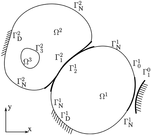
Figure 1. Schematic illustration of thegeometry and of the notation for the 2D case of N = 3 subdomains in contact including a rigid obstacle.

Let ℂ⁽ⁱ⁾ denote the elastic stiffness tensor of subdomain Ωⁱ, uⁱ(x, t) the time dependent displacements on Ωⁱ, $e^i(u^i)=\frac{1}{2}{(▽u^i)}^T+▽u^i$ the small strain tensor, σⁱ(uⁱ) = ℂ⁽ⁱ⁾eⁱ(uⁱ) the stress tensor, pⁱ(uⁱ) = σⁱ(uⁱ)νⁱ the boundary tractions, ${\sigma }_n^i=p^i(u^i){\nu }^i$ and ${\sigma }_t^i=p^i(u^i){\tau }^i$ the normal and tangential component of boundary tractions, respectively.

Let ${\Gamma }_j^i\subset {\Gamma }^i$ denote the part of the boundary Γⁱ which possibly can contact with Ω^j (j = 0, …, N and j ≠ i), referred to as potential contact zone of Ωⁱ with Ω^j. We also consider a possible contact with a rigid obstacle on a part of Γⁱ denoted as ${\Gamma }_0^i$.

We assume that the rest of Γⁱ is partitioned into the Dirichlet and Neumann parts of the boundary, ${{\Gamma }_{\text{D}}}^i$ and ${{\Gamma }_{\text{N}}}^i$, respectively. Time-dependent boundary displacement and traction vectors, ${u_{\text{D}}}^i(x,t)$ and ${p_{\text{N}}}^i(x,t)$, are prescribed on ${{\Gamma }_{\text{D}}}^i$ and ${{\Gamma }_{\text{N}}}^i$, respectively. Thus, e.g., any admissible displacement uⁱ(x, t) on Ωⁱ has to be equal to the prescribed displacement ${u_{\text{D}}}^i(x,t)$ on ${{\Gamma }_{\text{D}}}^i$. Let

$\begin{array}{rc}{\Gamma }_{\text{D}}={\displaystyle \bigcup _{1\le i\le N}}{{\Gamma }_{\text{D}}}^i\mathrm{\text{and}}{\Gamma }_{\text{N}}={\displaystyle \bigcup _{1\le i\le N}}{{\Gamma }_{\text{N}}}^i.& (1)\end{array}$

In the simplest case of conforming or receding contact with a zero initial gap, ${\Gamma }_j^i$ can be equal to ${\Gamma }_i^j$, but in general, e.g., in the case of advancing contact or a positive gap, they do not coincide. The initial contact zone (in the undeformed configuration) between subdomains Ωⁱ and Ω^j, and also the active contact zone (the set of points on each subdomain which will enter in contact in the deformed configuration) both should be included in ${\Gamma }_j^i$ and ${\Gamma }_i^j$. Specially, ${\Gamma }_j^i$ and ${\Gamma }_i^j$ may be larger than ∂Ωⁱ∩∂Ω^j for modeling an advancing contact.

We assume that an intermediate contact surface, denoted as Γ_ij = Γ_ji, can be defined for each couple of potential contact zones, with one-to-one and onto (bijective) and continuous mappings (projections) between ${\Gamma }_j^i$, ${\Gamma }_i^j$ and Γ_ij. A discretized version of such mappings is briefly introduced in section 6. A recent comprehensive revision of different projection techniques for a general contact configuration can be found in Yastrebov (2013). Additionally a normal direction is defined at each point of Γ_ij by a unit normal vector ${\nu }_j^i(=-{\nu }_i^j)$ (outward with respect to Ωⁱ). Recall that all ${\Gamma }_j^i$, ${\Gamma }_i^j$ and Γ_ij are defined in the undeformed configuration. In the simplest case of conforming or receding contact with a zero initial gap, typically, ${\Gamma }_j^i={\Gamma }_i^j={\Gamma }_{ij}$.

The contact zone Γ_C in the present problem is defined by the union of all intermediate contact surfaces

$\begin{array}{rc}{\Gamma }_{\text{C}}={\displaystyle \bigcup _{0\le i<j\le N}}{\Gamma }_{ij}.& (2)\end{array}$

The initial normal distance (gap) between some points $x^i\in {\Gamma }_j^i$ and $x^j\in {\Gamma }_i^j$ corresponding each other by the above defined mappings is given by the scalar gap function $g_{ij}=(x^j-x^i){\nu }_j^i$ defined on the intermediate contact surface Γ_ij. A positive value of the gap function means an initial separation whereas a negative value means an initial overlapping between the bodies in contact. This gap function is denoted as g_n on Γ_C.

Similarly, we also define ${\left[u\right]}_{\text{ij}}=u^j(x^j)-u^i(x^i)$ on Γ_ij as the signed difference of displacements (displacement jump) between some points $x^i\in {\Gamma }_j^i$ and $x^j\in {\Gamma }_i^j$ corresponding each other by the above defined mappings. The normal and tangential components [u]_n and [u]_t on Γ_C, respectively, are defined as ${\left[u\right]}_{\text{n}}={\left[u\right]}_{\text{ij}}{\nu }_j^i$ and ${\left[u\right]}_{\text{t}}={\left[u\right]}_{\text{ij}}{\tau }_j^i$. According to this definition, [u]_n, referred to as opening, decreases when subdomains Ωⁱ and Ω^j are getting closer, and [u]_n+g_n ≥ 0 should hold. [u]_t is referred to as sliding. Therefore, ${\left[u\right]}_{\text{ij}}={\left[u\right]}_{\text{n}}{\nu }_j^i+{\left[u\right]}_{\text{t}}{\tau }_j^i$. In fact, the model does not depend on the chosen orientation, and indices i and j are omitted when displacement jump is defined on Γ_C. The relations between the components of the tractions and displacement jump on a unilateral contact surface are shown in Figure 2, which indicates that σ_n ≤ 0 if [u]_n+g_n = 0 (contact), no overlapping being allowed, whereas σ_n = 0 if [u]_n+g_n>0 (separation), and σ_t = 0 in both cases.

FIGURE 2

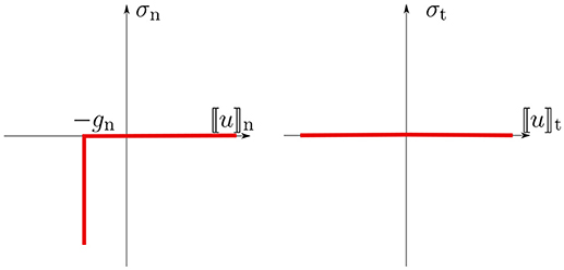
Figure 2. Constitutive relations for the unilateral frictionless contact considered.

The elastic strain energy $E$ stored in the volume $\Omega ={\bigcup }_{1\le i\le N}{\Omega }^i$ is

$\begin{array}{rc}E(u)={\displaystyle \sum _{i=1}^N}{E}^i(u^i)={\displaystyle \sum _{i=1}^N}{\displaystyle \underset{{\Omega }^i}{\int }}\frac{1}{2}{ℂ}^{(i)}{e}^i(u^i):e^i(u^i)\text{d}\Omega .& (3)\end{array}$

Then, the total potential energy functional, also referred to as the stored energy functional, is defined as

$\begin{array}{cc}\Pi (t,u)=\text{}\{\begin{array}{l}ℰ(u)-\mathcal{W}(t,u)\text{if }u=u_{\text{D}}\text{ on }{\Gamma }_{\text{D}},\hfill \\ {[u]}_{\text{n}}\ge -g_n\text{ on }{\Gamma }_{\text{C}},\hfill \\ \infty \text{\hspace{0.17em}elsewhere,}\hfill \end{array}& (4)\end{array}$

where, $W(t,u)=\sum _{i=1}^N\underset{{\Gamma }_{\text{N}}^i}{\int }{u}^i(x,t)·{p_{\text{N}}}^i(x,t)\text{d}S$ gives the work of external forces in Ω, the body forces being neglected for the sake of simplicity.

According to Fichera (1964, see also Kalker and Randen, 1972; Panagiotopoulos and Lazaridis, 1987), the minimizer u(t) of the total potential energy functional Π(t, u) at each time t is the solution of the unilateral frictionless contact considered.

Remark 1 (Adhesive unilateral frictionless contact). We refer to adhesive unilateral frictionless contact as the case where a continuous distribution of springs exists on an interface, i.e., a contact zone. The normal and tangential elastic stiffnesses of an interface, κ_n ≥ 0 and κ_t ≥ 0, respectively, may have different values (Figure 3). The interface response is considered frictionless, since no frictional dissipation of energy is considered, the tangent stiffness describing an adhesive elastic behavior. The elastic energy stored in such an adhesive interface (layer) is

$\begin{array}{rc}{E}_C(u)=E_{C\text{n}}(u)+E_{C\text{t}}(u),& (5)\end{array}$

where the components corresponding to the normal and tangential directions, respectively, are

$\begin{array}{cc}{ℰ}_{C\text{n}}(u)=\text{}\{\begin{array}{l}{\displaystyle {\int }_{{\Gamma }_{\text{C}}}\text{}}\text{}\frac{{\kappa }_{\text{n}}}{2}{[u]}_{\text{n}}{}^2\text{d}S\text{\hspace{0.17em}if[}u{]}_{\text{n}}\ge -g_n\text{ on }{\Gamma }_{\text{C}},\hfill \\ \infty \text{\hspace{0.17em}elsewhere,}\hfill \end{array}& (6)\end{array}$

and

$\begin{array}{rc}{E}_{C\text{t}}(u)={\displaystyle \underset{{\Gamma }_{\text{C}}}{\int }}\frac{{\kappa }_{\text{t}}}{2}{\left[u\right]}_{\text{t}}^2\text{d}S.& (7)\end{array}$

The total potential energy is augmented by the elastic energy stored in the adhesive interface layer giving

$\begin{array}{rc}\Pi (t,u)=E(u)+E_C(u)-W(t,u).& (8)\end{array}$

The relations between the components of the tractions and displacement jump on an adhesive interface layer are shown in Figure 3, which indicates that σ_n ≤ 0 if [u]_n + g_n = 0 (contact), whereas σ_n = κ_n[u]_n if [u]_n + g_n>0 (separation). Additionally, σ_t = κ_t[u]_t in shear. In this case, g_n represents the width of the adhesive layer. If [u]_n > 0 then the layer is under tensile stresses and we do not allow to break it, whereas if [u]_n < 0 then the layer is under compressive stresses and we assume a linear behavior until the two domains enter in contact, no overlapping being allowed.

FIGURE 3

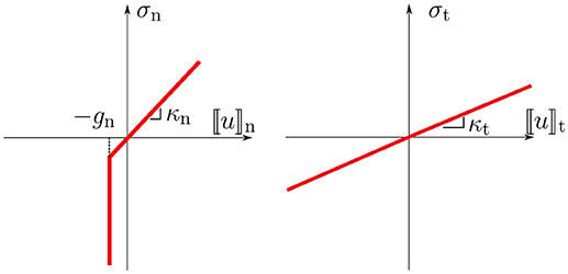
Figure 3. Constitutive relations for the adhesive unilateral contact considered.

It is easy to realize, that for vanishing interface stiffnesses, κ_n → 0 and κ_t → 0, the above described Signorini unilateral contact model is recovered, cf. Figures 2, 3.

3. Energy Principles in Boundary Integral Forms

For given body forces Fⁱ in the elastic domain Ωⁱ, the following equilibrium condition holds:

$\begin{array}{l}-\mathrm{\text{div}}{\sigma }^i(u^i)=F^i\mathrm{\text{in}}{\Omega }^i,\end{array}$

which multiplied by some virtual displacement field ũⁱ and integrated by parts over Ωⁱ gives

$\begin{array}{rc}{\displaystyle \underset{{\Omega }^i}{\int }}{\sigma }^i(u^i):{ϵ}^i({ũ}^i)d\Omega -{\displaystyle \underset{{\Gamma }^i}{\int }}{\sigma }^i(u^i)·{\nu }^i{ũ}^{i}dx={\displaystyle \underset{{\Omega }^i}{\int }}{F}^i{ũ}^{i}d\Omega .& (9)\end{array}$

This expression may be seen as the principle of virtual work, for virtual displacements ũⁱ. The dependence of stresses and subsequently tractions on displacements is explicitly indicated in the notation used. By assuming zero body forces (Fⁱ = 0) (in the present work) and choosing ũⁱ = uⁱ, the volume integral in (3) is replaced by the boundary integral

$\begin{array}{rc}{E}^i(u^i)=\frac{1}{2}{\displaystyle \underset{{\Gamma }^i}{\int }}{u}^i{p}^i(u^i)\text{d}S.& (10)\end{array}$

Furthermore, the total potential energy for Ωⁱ is

$\begin{array}{rc}{\Pi }^i(t,u^i)=E^i(u^i)-{\displaystyle \underset{{{\Gamma }_{\text{N}}}^i}{\int }}{u}^i(x,t){p_{\text{N}}}^i(x,t)\text{d}S.& (11)\end{array}$

In order to formulate the problem as a quadratic programming problem involving boundary values only, we further proceed manipulating (11). Similar formulations may be found in Antes and Panagiotopoulos (1992) (see chapter 8), where also a proof of existence and uniqueness of solutions is provided, and in Aour et al. (2007), however without the extent and the analysis introduced in the present work.

In the following, the BVP for a sub-domain Ωⁱ is considered in a similar way as in Panagiotopoulos et al. (2013). Hereinafter in this section we will omit superindex i, for the sake of simplicity. Let u_η and p_η, respectively, denote the displacement and traction solutions of this BVP restricted to Γ_η, η = C, D and N, e.g. u_C = u|_ΓC and p_D = p|_ΓD. We study here a mixed-type operator ${M}$ which formally assigns (p_C, p_D, u_N) to the known boundary data (u_C, u_D, p_N) of the original BVP $P$^O shown in Figure 4, and may be partitioned using the following block structure as

$\begin{array}{rc}\left(\begin{array}{c}{p}_{\text{C}}\\ p_{\text{D}}\\ u_{\text{N}}\end{array}\right)=\left(\begin{array}{ccc}{{M}}_{\mathrm{\text{CC}}}& {{M}}_{\mathrm{\text{CD}}}& {{M}}_{\mathrm{\text{CN}}}\\ {{M}}_{\mathrm{\text{DC}}}& {{M}}_{\mathrm{\text{DD}}}& {{M}}_{\mathrm{\text{DN}}}\\ {{M}}_{\mathrm{\text{NC}}}& {{M}}_{\mathrm{\text{ND}}}& {{M}}_{\mathrm{\text{NN}}}\end{array}\right)\left(\begin{array}{c}{u}_{\text{C}}\\ u_{\text{D}}\\ p_{\text{N}}\end{array}\right).& (12)\end{array}$

The columns of the aforementioned block operator ${M}$ are associated to the sub-problems $P$^η defined in Figure 4. The displacement solution of a subproblem $P$^η is denoted as u^η. From the principle of superposition the displacement solution of the full problem $P$^O may be reconstructed by the sum:

$\begin{array}{rc}u=u^{\text{C}}+u^{\text{D}}+u^{\text{N}}.& (13)\end{array}$

In view of (10) and (11), the total potential energy for the mixed type BVP $P$^O may be written in an expanded form as

$\begin{array}{rc}\Pi (t,u)=\frac{1}{2}{\displaystyle \underset{{\Gamma }_{\text{C}}}{\int }}{u}_{\text{C}}(u)p_{\text{C}}(u)\text{d}S+\frac{1}{2}{\displaystyle \underset{{\Gamma }_{\text{D}}}{\int }}{u}_{\text{D}}{p}_{\text{D}}(u)\text{d}S-\frac{1}{2}{\displaystyle \underset{{\Gamma }_{\text{N}}}{\int }}{u}_{\text{N}}(u)p_{\text{N}}\text{d}S,& (14)\end{array}$

where we tacitly assumed that u fulfills the Dirichlet and Neumann boundary conditions. By substituting the unknown data for problem $P$^O from (12), the total potential energy can be written as

$\begin{array}{r}\Pi (t,u_{\text{C}})=\frac{1}{2}{\displaystyle \underset{{\Gamma }_{\text{C}}}{\int }}{u}_{\text{C}}{{M}}_{\mathrm{\text{CC}}}{u}_{\text{C}}\text{d}S+{\displaystyle \underset{{\Gamma }_{\text{C}}}{\int }}{u}_{\text{C}}{{M}}_{\mathrm{\text{CD}}}{u}_{\text{D}}\text{d}S+{\displaystyle \underset{{\Gamma }_{\text{C}}}{\int }}{u}_{\text{C}}{{M}}_{\mathrm{\text{CN}}}{p}_{\text{N}}\text{d}S\\ +{\displaystyle \underset{{\Gamma }_{\text{D}}}{\int }}{u}_{\text{D}}{{M}}_{\mathrm{\text{DC}}}{u}_{\text{C}}\text{d}S+{\displaystyle \underset{{\Gamma }_{\text{D}}}{\int }}{u}_{\text{D}}{{M}}_{\mathrm{\text{DD}}}{u}_{\text{D}}\text{d}S+{\displaystyle \underset{{\Gamma }_{\text{D}}}{\int }}{u}_{\text{D}}{{M}}_{\mathrm{\text{DN}}}{p}_{\text{N}}\text{d}S& (15)\end{array}$

From (15) it is clear, that since, at time t, u_D and p_N are a priori known prescribed values, the total potential energy is actually a function of only the contact displacements u_C. We further modify (15) in order to keep the unknown contact displacements u_C in the integrals on Γ_C part only, by utilizing the following reciprocity relations between the elastic solutions of $P$^C and $P$^N

$\begin{array}{rc}-{\displaystyle \underset{{\Gamma }_{\text{N}}}{\int }}{p}_{\text{N}}{{M}}_{\mathrm{\text{NC}}}{u}_{\text{C}}\text{d}S={\displaystyle \underset{{\Gamma }_{\text{C}}}{\int }}{u}_{\text{C}}{{M}}_{\mathrm{\text{CN}}}{p}_{\text{N}}\text{d}S& (16)\end{array}$

as well as between the solutions of $p$^C and $p$^D,

$\begin{array}{rc}{\displaystyle \underset{{\Gamma }_{\text{D}}}{\int }}{u}_{\text{D}}{{M}}_{\mathrm{\text{DC}}}{u}_{\text{C}}\text{d}S={\displaystyle \underset{{\Gamma }_{\text{C}}}{\int }}{u}_{\text{C}}{{M}}_{\mathrm{\text{CD}}}{u}_{\text{D}}\text{d}S.& (17)\end{array}$

A similar reciprocal relation holds true for the solutions of $P$^N and $P$^D,

$\begin{array}{rc}-{\displaystyle \underset{{\Gamma }_{\text{N}}}{\int }}{p}_{\text{N}}{{M}}_{\mathrm{\text{ND}}}{u}_{\text{D}}\text{d}S={\displaystyle \underset{{\Gamma }_{\text{D}}}{\int }}{u}_{\text{D}}{{M}}_{\mathrm{\text{DN}}}{p}_{\text{N}}\text{d}S.& (18)\end{array}$

Notice a somewhat surprising presence of the negative sign in (16) and (18). It should be mentioned that (16), (17) and (18) hold only approximately in the case of numerical solution of the pertinent problems.

FIGURE 4

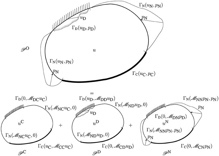
Figure 4. Solution of a mixed BVP $p$^O for a single elastic domain given as a superposition of the solutions of the three sub-problems $p$^C, $p$^D and $p$^N.

Substituting the relations (16) and (17) into the expression (15) gives

$\begin{array}{c}\Pi (t,u_{\text{scC}})={\displaystyle {\int }_{{\Gamma }_{\text{scC}}}\text{}}\text{}{u}_{\text{scC}}(\frac{1}{2}{ℳ}_{\text{scCC}}{u}_{\text{scC}}+{ℳ}_{\text{scCD}}{u}_{\text{scD}}+{ℳ}_{\text{scCN}}{p}_N)ds+\frac{1}{2}{\displaystyle {\int }_{{\Gamma }_{\text{scD}}}\text{}}\text{}{u}_{\text{scD}}{ℳ}_{\text{scDD}}{u}_{\text{scD}}ds\\ +\frac{1}{2}{\displaystyle {\int }_{{\Gamma }_{\text{scD}}}\text{}}\text{}{u}_{\text{scD}}{ℳ}_{\text{scDN}}{p}_{N}ds-\frac{1}{2}{\displaystyle {\int }_{{\Gamma }_{\text{scD}}}\text{}}\text{ }ds{ℳ}_{\text{scND}}{u}_{\text{scD}}ds-\frac{1}{2}{\displaystyle {\int }_{{\Gamma }_{\text{scD}}}\text{}}\text{}{p}_N{ℳ}_{\text{scNN}}{p}_{N}ds& (19)\end{array}$

The present problem can be defined now in an explicit form as a quadratic programming problem. By observing here that the last four integrals in (19) are constant with respect to u_C, we may omit them in the minimization procedure since they do not have influence on the minimizer of the total potential energy. This leads to the following simplified expression including only the variable part of the total potential energy functional (for the sake of simplicity the notation of this functional is kept the same):

$\begin{array}{cc}\Pi (t,u_{{}_{\text{C}}})=\underset{\mathcal{A}(u_{{}_{\text{C}}})}{\underbrace{\frac{1}{2}\text{}{\displaystyle {\int }_{{\Gamma }_{\text{C}}}{u}_{{}_{\text{C}}}}{ℳ}_{\text{CC}}{u}_{{}_{\text{C}}}dS}}+\underset{-b(t,u_{{}_{\text{C}}})}{\underbrace{{\displaystyle {\int }_{{\Gamma }_{\text{C}}}}{u}_{{}_{\text{C}}}({ℳ}_{\text{CD}}{u}_{\text{D}}(t)+{ℳ}_{\text{CN}}{p}_N(t))dS}}& (20)\end{array}$

After a suitable discretization of u_C by means of a linear combination of standard vector shape-functions

$\begin{array}{rc}{u}_{\text{C}}(x)={\displaystyle \sum _{i=1}^{M_{\mathrm{\text{C}}}}}{\varphi }_i(x){\xi }_i& (21)\end{array}$

where M_C is the number of displacement degrees-of-freedom (DOFs), typically nodal values of displacement components, on the contact zone Γ_C. The expression in (20) may be rewritten as an algebraic representation of the corresponding quadratic function

$\begin{array}{rc}\Pi (t,\xi )=\frac{1}{2}{\xi }^T\text{A}\xi -{\xi }^T\text{b}(t),& (22)\end{array}$

where ξ is a vector of the nodal displacements u_C on Γ_C, and A is a kind of the boundary stiffness matrix associated to Γ_C.

Recall that (20), (21) and (22) refer to a single domain. Then, the total potential energy for the assemblage of N bodies is defined as follows

$\begin{array}{rc}\Pi ={\displaystyle \sum _{i=1}^N}{\Pi }^i(t,{u_{\text{C}}}^i).& (23)\end{array}$

This leads to the fact that the algebraic representation of the total potential energy Π for the assemblage in of N bodies in (23) adopts the same form as in (22), however, with the matrix A defined as a block diagonal matrix formed by the individual matrices Aⁱ for subdomains Ωⁱ,

$\begin{array}{rc}\text{A}=\mathrm{\text{block-diag}}\left\{{\text{A}}^1,\dots ,{\text{A}}^N\right\},& (24)\end{array}$

and similarly the vector b defined as a block vector by formed by the individual vectors bⁱ for Ωⁱ

$\begin{array}{rc}{\text{b}}^T=\left\{{({\text{b}}^1)}^T,\dots ,{({\text{b}}^N)}^T\right\}.& (25)\end{array}$

4. Boundary Element Method

As can be seen, the possibilities for a numerical implementation of the above framework are quite wide, the key issue is the approximation of the operators ${{M}}_{\mathrm{\text{CC}}}^i$, ${{M}}_{\mathrm{\text{CD}}}^i$ and ${{M}}_{\mathrm{\text{CN}}}^i$ for each subdomain Ωⁱ. Several numerical methods, such as the finite element method (FEM) or boundary element method (BEM), may be utilized. Since the adjacent bodies represented by Ωⁱ(i =, 1, …, N), possibly in contact, are linearly elastic, collocation BEM or symmetric Galerkin BEM provide an intrinsic advantage herein. In the present implementation, the collocation BEM has been adopted.

The BEM is closely related to the map between the prescribed boundary conditions in displacements or tractions and the unknown boundary displacements or tractions. In pure Dirichlet and Neumann boundary-value problems (BVPs), these maps are called Steklov-Poincaré and Poincaré-Steklov maps, respectively, and BEM can be considered as an approach to discretize these maps. In the present computational procedure, the role of the BEM analysis, applied to each subdomain Ωⁱ separately (which, in fact, makes this problem very suitable for parallel computers), is to solve the corresponding BVPs on each Ωⁱ. For this goal, we numerically solve the Somigliana displacement identity (see París and Cañas, 1997; Aliabadi, 2002),

$\begin{array}{rc}{c}_{ml}^i(y)u_m^i(y)+{\displaystyle \underset{{\Gamma }^i}{\int }}-u_m^i(x)T_{ml}^i(x,y)\text{d}{S}_x={\displaystyle \underset{{\Gamma }^i}{\int }}{p}_m^i(x)U_{ml}^i(x,y)\text{d}{S}_x,& (26)\end{array}$

where y ∈ Γⁱ and $u_m^i(x)$ and $p_m^i(x)$ denote the m-component of displacement and traction vectors, respectively. The weakly singular integral kernel $U_{ml}^i(x,y)$, two-point tensor field, given by the Kelvin fundamental solution (free-space Green's function) represents the displacement at x in the m-direction originated by a unit point force at y in the l-direction in the unbounded linear-elastic medium defined by ℂ⁽ⁱ⁾. The strongly singular integral kernel $T_{ml}^i(x,y)$, two-point tensor field, represents the corresponding tractions at x in the m-direction. The coefficient-tensor $c_{ml}^i(y)$ of the free-term is a function of the local geometry of the boundary Γⁱ at y, and may be evaluated by a closed analytical formula for isotropic elastic solids (see Mantič, 1993). The symbol $\sout{\int }$ in (26) stands for the Cauchy principal value of an integral.

Consider a discretization of the boundary Γⁱ by a boundary element mesh, which is also used to define a suitable discretization of boundary displacements uⁱ(x) and tractions pⁱ(x) by interpolations of their nodal values along Γⁱ denoted as uⁱ and pⁱ, respectively. By imposing (collocating) the Somigliana identity (26) at all boundary nodes (called collocation points) we set the BEM system of linear equations for Γⁱ, typically written as Hⁱ uⁱ = Gⁱ pⁱ (see París and Cañas, 1997; Aliabadi, 2002). The solution of this system provides the unknown nodal values of boundary displacements and tractions.

In the present computational implementation of BEM, straight elements with piecewise linear continuous interpolation for displacements and piecewise linear (possibly discontinuous) interpolation for tractions are adopted, respectively. On the Γ_C part of the boundaries, usually standard continuous interpolation for tractions is used.

In the context of BEM, operators ${{M}}_{\text{IJ}}^i$, of (12), with I, J = C, D and N do not need to be explicitly constructed, since what we actually need are the resultant tractions or displacements for each sub-problem, as also shown in Figure 4. Thus, we need to solve these three sub-problems for each subdomain Ωⁱ by BEM.

5. Explicit Computation of the Matrix A and Vector B

The matrix A in (22) has the physical meaning of a boundary stiffness matrix for a subdomain. Several established techniques may be utilized for its computation, a survey of such techniques based on the BEM may be found in Hartmann (1981) and Tullberg and Bolteus (1982). Hereinafter a new methodology for computing A is introduced. This methodology is consistent with the present energetic approach and leads directly to a symmetric form of A. From (20), the quadratic form $A$ and linear form b write as

$\begin{array}{rcl}A(\xi )& =\frac{1}{2}{\xi }^T\text{A}\xi =\frac{1}{2}{\displaystyle \sum _{i,j=1}^{M_{\mathrm{\text{C}}}}}{a}_{ij}{\xi }_i{\xi }_j,& (27)\end{array}$

$\begin{array}{rcl}b(\xi )& ={\xi }^T\text{b}={\displaystyle \sum _{i=1}^{M_{\mathrm{\text{C}}}}}{b}_i{\xi }_i,& (28)\end{array}$

with M_C being the number of displacement DOFs on the contact zone Γ_C.

Choosing ξ⁽ⁱ⁾ defined as

$\begin{array}{rc}{\xi }_i^{(i)}=1,{\xi }_j^{(i)}=0,\forall j\ne i,& (29)\end{array}$

then (27) simplifies to

$\begin{array}{rc}A({\xi }^{(i)})=\frac{1}{2}{a}_{ii}\to a_{ii}={\displaystyle \sum _{k,l=1}^{M_{\mathrm{\text{C}}}}}{\xi }_k^{(i)}{\xi }_l^{(i)}{\displaystyle \underset{{\Gamma }_{\text{C}}}{\int }}{\varphi }_k{{M}}_{\mathrm{\text{CC}}}{\varphi }_l\text{d}S.& (30)\end{array}$

Solving the above problem $P$^C by BEM sequentially for all i = 1, …, M_C, and by utilizing the first integral of (20), we may compute all the diagonal components a_ii of matrix A.

Furthermore, in order to compute the non-diagonal components a_ij we choose ξ^{(i, j)} defined as

$\begin{array}{rc}{\xi }_i^{(i,j)}={\xi }_j^{(i,j)}=1,{\xi }_m^{(i,j)}=0,\forall m\ne i,j,& (31)\end{array}$

then, similarly to (30),

$\begin{array}{rcl}A({\xi }^{(i,j)})& =\frac{1}{2}(a_{ii}+a_{jj}+a_{ij}+a_{ji})=\frac{1}{2}{a}_{ii}+\frac{1}{2}{a}_{jj}+a_{ij}& (32)\end{array}$

$\begin{array}{rc}=\frac{1}{2}{\displaystyle \sum _{k,l=1}^{M_{\mathrm{\text{C}}}}}{\xi }_k^{(i,j)}{\xi }_l^{(i,j)}{\displaystyle \underset{{\Gamma }_{\text{C}}}{\int }}{\varphi }_k{{M}}_{\mathrm{\text{CC}}}{\varphi }_l\text{d}S.& (33)\end{array}$

Having computed the diagonal elements a_ii we may compute from the last equation also the non-diagonal elements, considering a_ij = a_ji, by

$\begin{array}{rc}{a}_{ij}=\frac{1}{2}\left({\displaystyle \sum _{k,l=1}^{M_{\mathrm{\text{C}}}}}{\xi }_k^{(i,j)}{\xi }_l^{(i,j)}{\displaystyle \underset{{\Gamma }_{\text{C}}}{\int }}{\varphi }_k{{M}}_{\mathrm{\text{CC}}}{\varphi }_l\text{d}S-a_{ii}-a_{jj}\right).& (34)\end{array}$

Similarly, solving the above problems $P$^D and $P$^N by BEM, the computation of vector b is carried out by using the first set of vectors ξ⁽ⁱ⁾ and computed by the second integral in (20), and its components are given as

$\begin{array}{l}b({\xi }^{(i)})=b_i\to b_i=-{\displaystyle \sum _{k=1}^{M_{\mathrm{\text{C}}}}}{\xi }_k^{(i)}{\displaystyle \underset{{\Gamma }_{\text{C}}}{\int }}{\varphi }_k({{M}}_{\mathrm{\text{CD}}}{u}_{\text{D}}+{{M}}_{\mathrm{\text{CN}}}{p}_{\text{N}})\text{d}S.\end{array}$

A more direct relation of the matrix A to a respective stiffness matrix could be understood for the case of a single domain where the whole boundary Γ coincides with Γ_C (see also section 10). Although by the procedure described above a direct symmetric stiffness matrix may be constructed, this matrix was found to lack the properties of equilibrium and rigid motion representation, which are satisfied only approximately and although after a mesh refinement their fulfillment is improved nevertheless they are not fully satisfied. A further detailed study of the properties of this matrix is given in section 10. Additionally in section 9, some alternative modified procedure in order to construct a non-symmetric matrix A together with the reasoning of its necessity is proposed and discussed.

6. The Contact Description Via Interface Elements

Usually, a unilateral frictionless contact law is defined by a geometric condition of non-penetration (also referred to as compatibility of displacements), a static condition of no tension and no friction and equilibrium of forces (see Renaud and Feng, 2003). In the context of small displacements deformation, we may write the non-penetration condition in the normal direction associated to the surfaces under contact (see below). The exact portion of the boundaries Ωⁱ and Ω^j which will really contact, the so-called active contact zone, is a priori unknown, for this reason initially we consider ${\Gamma }_j^i$ and ${\Gamma }_i^j$ as potential contact boundaries, which should include the points of the active contact zone (see Figure 1).

The establishment of relations that impose the non-penetration also referred to as Signorini condition, is one of the most crucial parts of the present formulation. Some of the BEM formulations for contact problems enforce compatibility of displacements on one of the domains, while on the other the equilibrium is enforced (cf. Blázquez et al., 1998b; Graciani et al., 2005). These equilibrium conditions might be given in weak sense instead of their strong form (see Blázquez et al., 1998a). In the present methodology only compatibility conditions are enforced between the bodies in potential contact, by establishing the non-penetration condition which include the evaluation of the displacement jump [u] and gap g_n along Γ_C, while the equilibrium of contact tractions arises through the enforcement of the principle of minimum of the total potential energy.

The interconnection of the subdomains as well as the consideration of Signorini kinematical conditions is succeeded by the intermediate surface discretized by interface elements, as shown in Figure 5A. Let us consider an intermediate surface between two bodies. The gap g_n, at this surface may be considered as finite or zero valued. For each node of the interface elements we define a local reference system and each relative displacement may have an opening (normal) and sliding (tangential) component. In the case of contact problems of two deformable bodies where only small changes in the geometry are assumed and also the mesh of each elastic domain is a conforming one, it is possible to incorporate the contact constraints on a purely nodal basis. However, for the general case of nodes being arbitrarily distributed along the potential contact zone between two bodies, which can occur, e.g., when automatic meshing is used for these bodies, further consideration must be taken into account in the definition of Signorini contact conditions. Such techniques have been developed in the case of BEM in Blázquez et al. (1998b), Graciani et al. (2005), Blázquez et al. (2006), Graciani et al. (2009), and Vodička (2000). Nevertheless, the necessity of non-conforming algorithms may also occur in small displacements contact problems and conforming discretizations as shown in Blázquez and París (2009). The non-penetration conditions for the case of non-conforming mesh are considered in the normal direction of the intermediate surface at interface nodes. Each interface node, related to a pair of the adjacent BEM node and boundary point, the latter may coincide with a BEM node or just be located on a BEM element as depicted in Figure 5B. For the latter case, the displacements of the boundary point are computed by the respective displacements of the nodes of this BEM element. The Signorini conditions, that also take into account a possible initial gap (or a finite thickness of the adhesive layer) are imposed on the normal displacements of those pairs. We will write here the conditions taken into account for two different cases referring to Figure 5B. In the first case, the BEM node is denoted as i_m (main) and the adjacent boundary point coincides with another BEM node denoted as i_s (secondary), and the following condition is taken into account:

$\begin{array}{rc}{\left[u^m(i_m)-u^s(i_s)\right]}_n\ge -g_n(i).& (35)\end{array}$

In the next case, the BEM node is denoted as l_m (main) and the adjacent boundary point, denoted as l_s (secondary), does not coincide with any BEM node (see Figure 5B), then the following condition is taken into account:

$\begin{array}{r}{\left[u^m(l_m)-u^s(l_s)\right]}_n\ge -g_n(l)\Rightarrow \end{array}$

$\begin{array}{rc}{\left[u^m(l_m)-\frac{L_{ln}}{L_{kn}}{u}^s(k_s)-\frac{L_{kl}}{L_{kn}}{u}^s(n_s)\right]}_n\ge -g_n(l).& (36)\end{array}$

The entire set of such equations may be given in a more compact algebraic form in terms of new variables

$\begin{array}{rc}{f}_i=c_{ij}{u}_j,& (37)\end{array}$

where f_i is given by the i^th constraint expression, c_ij is the so-called constraint matrix and u_j are the components of normal displacements on the potential contact zone, which are the only variables included in the minimization procedure for the frictionless contact as will be shown in the following section. The inclusion of the tangential components of displacements on the contact zone in the case of adhesive frictionless contact is straightforward and will be omitted here for the sake of brevity.

FIGURE 5

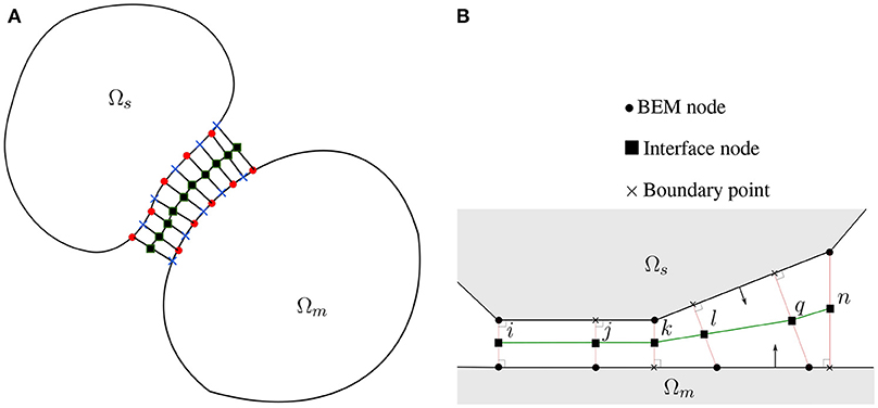
Figure 5. (A) Interface elements constructed on an intermediate surface between two domains under possible contact, and (B) main and secondary elastic domains, corresponding nodes and interface elements.

7. Minimization of Total Potential Energy

As shown in section 2, the contact problem can be formulated as a minimization problem of the total potential energy functional defined in (4). In section 3 appropriate boundary integral forms of this functional were derived in order to generate a pure boundary value problem, as in (10) or (11), which was further manipulated in order to derive a quadratic functional in (20). In section 1 it was assumed, that the problem is a quasi-static one (neglecting inertial and viscous effects), introducing by this way a (pseudo)time variable t into the stored energy functional in (4). Finally, in section 6 it was shown that in order to define the minimization problem as a simple bound constrained one it is advantageous to work with variables f_i defined by (37). Making a time discretization by adopting, for simplicity only and without loss of generality, an equidistant partition of [0, T] with a fixed time-step τ > 0, assuming T/τ ∈ ℕ, the minimization of the total potential energy functional defined in (4) leads to the following (formally written) recursive minimization problem:

$\begin{array}{cc}\begin{array}{l}\text{minimize}{ℱ}^k(f)=\Pi (k\tau ,u(f))\hfill \\ \text{subject to\hspace{0.17em}}f\ge -g\hfill \end{array}\}& (38)\end{array}$

to be solved successively for k = 1, …, T/τ. Here, f is the vector defined by Equation (37) and g the vector that contains the gap values.

For the numerical resolution of the above minimization problem there are two possible approaches, always taking into account the transformation in (37), the first is to directly minimize the objective function of type given in (11). In this case we may use a general algorithm for bound-constraint optimization problems, such as the L-BFGS-B by Zhou et al. (1997). However, it is usually advantageous to solve the problem as a quadratic one and for this reason we utilize (23) or its algebraic form as in (22). A variety of algorithms for quadratic programming may be found in Dostál (2009). Notice that, using the algebraic form of (22), the problem may be stated as a Linear Complementarity Problem (LCP), cf. (Gakwaya et al., 1992; Stavroulakis and Antes, 1997), and may be solved, for example, by Lemke's algorithm. For the present EC-BEM computer implementation, we use a modified conjugate gradient method which does not need an explicit form of matrix A and vector b in (22) and directly minimizes (23). Its pseudocode is given in Table 1. Nevertheless, also the conventional conjugate gradient method is reproduced in Table 2 following Dostál (2009). A further discussion on differences between these two variants of the conjugate gradient algorithm is given in section 9.

TABLE 1

Table 1. (M1) Conjugategradient method (CG) adapted for EC–BEM.

TABLE 2

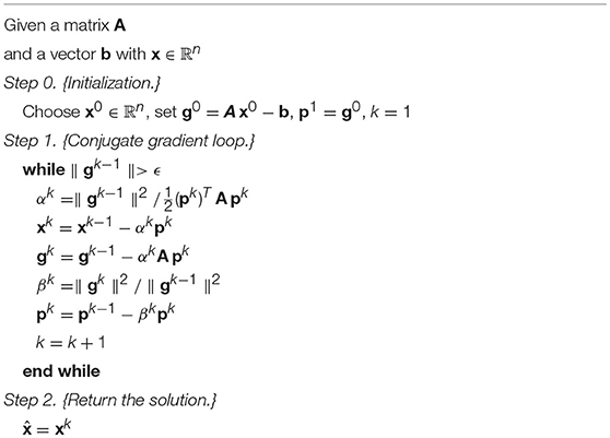
Table 2. (M2) Conjugate gradient method (CG).

Regardless of the minimization algorithm we use, except if it would be a derivative free algorithm, we always need to calculate the partial derivatives of the potential energy Π. An alternative to compute these derivatives would be to use finite differences but such an approach was proved to be extremely time consuming. For this reason, we set up an analytical computation of derivatives of Π. By applying the chain rule of differentiation we obtain

$\begin{array}{rc}\frac{\partial \Pi }{\partial f_i}=\frac{\partial \Pi }{\partial u_j}\frac{\partial u_j}{\partial f_i},& (39)\end{array}$

and by inverting (37)

$\begin{array}{rc}{u}_i=r_{ij}{f}_j,& (40)\end{array}$

where $r_{ij}={(c^{-1})}_{ij}$, which substituted into (39) leads to

$\begin{array}{rc}\frac{\partial \Pi }{\partial f_i}=\frac{\partial \Pi }{\partial u_j}{r}_{ji}.& (41)\end{array}$

Having established the quadratic formula for (23), the derivatives in (41) can be easily defined. In section 8 we give a more general treatment on how to define the derivatives of the total potential energy (11) with respect to a displacement component.

8. Derivatives of the Total Potential Energy with Respect to Displacements

When the minimization problem (38) is formulated as a quadratic programming problem, derivatives of Π, for a single domain, with respect to the degrees-of-freedom (DOFs) of displacements u_C on the potential contact zone can be easily computed.

However, we might also treat the minimization problem as a general one. In that case we might need the derivatives of Π as given in (11). The total potential energy functional Π from (11), for a single domain, is a function of u defined on Γ, but it also contains the tractions p, which are functions of displacements, i.e., p(u), and for this reason the derivatives with respect to u cannot be computed in a straightforward manner. The displacement and traction variables, according to the BEM formulation, are discretized for x ∈ Γ as

$\begin{array}{rcl}u(x)& ={\displaystyle \sum _i}{\varphi }_i(x)u_i,& (\mathrm{42a})\end{array}$

$\begin{array}{rcl}p(x)& ={\displaystyle \sum _i}{\psi }_i(x)p_i,& (\mathrm{42b})\end{array}$

where ϕ_i(x) and ψ_i(x) are the vector shape-functions associated to DOFs i defining the boundary values of displacements and tractions, respectively. The partial derivative of the total potential energy with respect to a DOF u_i is the functional derivative with the test function being the vector shape-function ϕ_i associated to this DOF

$\begin{array}{rc}\frac{\partial \Pi (u)}{\partial u_i}={\displaystyle \underset{\delta u_i\to 0}{lim}}\frac{\Pi (u+{\varphi }_i(x)\delta u_i)-\Pi (u)}{\delta u_i},& (43)\end{array}$

where utilizing (11) leads to

$\begin{array}{l}\Pi \left(u+{\varphi }_i(x)\delta u_i\right)=\\ \frac{1}{2}{\displaystyle {\int }_{\Gamma }p}(u(x)+{\varphi }_i(x)\delta u_i)\left(u(x)+{\varphi }_i(x)\delta u_i\right)\text{d}x\\ -{\displaystyle {\int }_{{\Gamma }_N}(}u(x)+{\varphi }_i(x)\delta u_i)p_N\text{d}x=\\ \frac{1}{2}{\displaystyle {\int }_{\Gamma }(p(u(x))u(x)+p(u(x)){\varphi }_i(x)\delta u_i+p({\varphi }_i(x))u(x)\delta u_i}\\ +p({\varphi }_i(x))\delta u_i^2{\varphi }_i(x))\text{d}x\\ -{\displaystyle {\int }_{{\Gamma }_N}(}{p}_{N}u(x)+p_N{\varphi }_i(x)\delta u_i)\text{d}x,& (44)\end{array}$

where the linearity of the tractions p(u) with respect to the displacements u was used. Note that the term in the above integral which includes a higher order term $(\delta u_i^2)$ is dropped out in the limit in (43). Introducing the above expression in (43) leads to

$\begin{array}{l}\frac{\partial \Pi (u)}{\partial u_i}=\frac{1}{2}{\displaystyle {\int }_{\Gamma }(}p(u(x)){\varphi }_i(x)+p({\varphi }_i(x))u(x))dx\\ -{\displaystyle {\int }_{{\Gamma }_N}{p}_N}{\varphi }_i(x)dx={\displaystyle {\int }_{\Gamma }p}(u(x)){\varphi }_i(x)dx\\ -{\displaystyle {\int }_{{\Gamma }_N}{p}_N}{\varphi }_i(x)dx,& (45)\end{array}$

where the reciprocity between the two states: ((u(x), p(u(x))) and (ϕ_i(x), pϕ_i(x))) was used. Equation (45), after introducing also (42b) (actually the tractions computed by the (numerical) solution of the Dirichlet problem with the boundary conditions given by u on Γ), will result in the following formula, for a single domain, appropriate for the EC-BEM implementation:

$\begin{array}{rc}\frac{\partial \Pi (u)}{\partial u_i}={\displaystyle \underset{\Gamma }{\int }}{\psi }_j(x){\varphi }_i(x)p_j\text{d}x-{\displaystyle \underset{{\Gamma }_{\text{N}}}{\int }}{\psi }_j(x){\varphi }_i(x)p_{\text{N}j}\text{d}x.& (46)\end{array}$

The integration in (46) does not need to be extended all over the boundary Γ since ψ_j and ϕ_i are local vector shape-functions whose support is given only by the boundary elements associated to the DOFs j and i, respectively. Taking also into account that, for the minimization problem under study, the relevant DOF are associated to Γ_C and their support is a part of Γ_C, supp ϕ_i⊂Γ_C, Equation (46) can be further simplified as

$\begin{array}{rc}\frac{\partial \Pi (u)}{\partial u_i}={\displaystyle \underset{\Gamma }{\int }}{\psi }_i(x){\varphi }_i(x)p_i\text{d}x.& (47)\end{array}$

This expression gives the relevant numerically computed gradient of the potential energy in the present problem in terms of the numerically computed boundary tractions on Γ_C.

9. A Critical Comparison of Algorithms M1 and M2

In Tables 1, 2 of section 7, two variants of the conjugate gradient method considered, M1 and M2, respectively, were described by pseudocodes, where M2 is the original version introduced by Dostál (2009). The main difference between these two variants, is that in M1 we do not explicitly calculate the matrix A, since instead of using the vector-matrix-vector product $\frac{1}{2}{\text{x}}^T\text{A}\text{x}$ and the matrix-vector product Ax, we use the quadratic form $A$ (x) and the derivative $A$ ′(x). In reference to M2, we initially need to compute the matrix A, as it is described in section 5 (actually it is the Step 0 in Table 2), which might be time consuming, but then the rest of the procedure, that is actually the conjugate gradient loop, showed to be fast enough. On the contrary, for M1 the initialization (Step 0) is direct and fast, however each time we need to compute the value of the quadratic form $A$ (x) and its derivative $A$ ′(x), that is in each k^th step of the conjugate gradient loop (Step 1 in Table 1), a BEM solution is required. Nevertheless, the influence BEM matrices need to be computed only once, for all the iterations and time steps. Additionally, having decomposed the matrix of the linear algebraic system of equations produced by BEM (e.g., by LU- or QR-decomposition), each time that the solution of this system is required, only a back-substitution takes place.

Details of the algorithms for constrained minimization problems can be found in Dostál (2009). In this work, for both variants of the conjugate algorithms, we employed Polyak's algorithm for bound constrained minimization (Algorithm 5.2 in Dostál, 2009), for which the number of iterations is bounded by Ñ = n²2ⁿ, while for the standard conjugate gradient algorithm by N = n, with n being the number DOFs, i.e., the order of the matrix A. However, according to Dostál (2009), this bound for Polyak's algorithm may be considered too pessimistic.

It was found, in this work, that in M2 the usage of the symmetric matrix described in section 5, leads to exactly the same results for the energy calculation as in M1, i.e., $A(\text{x})=\frac{1}{2}{\text{x}}^T\text{A}\text{x}$. However, the accuracy of the results for displacements and tractions was worse in M2 using the symmetric matrix than in M1, especially for points near a change of boundary condition type (that is from Γ_C to Γ_N). Previously, similar observations were made in BEM by de Paula and Telles (1989) and Tullberg and Bolteus (1982), when the symmetric stiffness matrices was chosen instead of the non-symmetric one. We conclude that the source of this lose of accuracy in our context is because the numerically computed derivatives (gradient) of the quadratic form used in M1 and M2 may be quite different, i.e., $A$ ′(x)≠Ax, when the symmetric matrix A is used in M2 and if in M1, instead of computing explicitly the gradient of the quadratic form, we use its expression in terms of the boundary tractions according to section 8. In order to overcome this difficulty in M2 application we proceed to construct a consistent non-symmetric matrix $\tilde{\text{A}}$ for its usage in M2.

In Antes and Panagiotopoulos (1992), it is claimed that the stiffness matrix constructed by BEM should be symmetric due to Betti's theorem, and not because of the numerical method used to compute the unit displacement response. This might be equivalent with our consideration here, that the reciprocity statements in the context of a numerical implementation of BEM are only approximately valid. In order to construct the non-symmetric matrix $\tilde{\text{A}}$, we solve by BEM a problem, for each ith DOF of displacements on Γ_C, such that each time this is the only non zero component and equal to the unit value. The ith column of the $\tilde{\text{A}}$ matrix consists of the derivatives $\frac{\partial A}{\partial u_j}$, with u_j being a DOF of displacements on Γ_C.

It can be shown, and also it was numerically verified, that the matrix A of section 5, is the symmetric part of matrix $\tilde{\text{A}}$ constructed here, i.e., $\text{A}=\frac{{\tilde{\text{A}}}^T+\tilde{\text{A}}}{2}$.

10. Properties of the Symmetric and Non-Symmetric BEM Matrices: A and $\tilde{\text{a}}$

As mentioned in Table 2, the matrix A is assumed to be symmetric and positive definite. However, it is well known that it is possible to apply the conjugate gradient method of Hestenes and Stiefel (1952) also to non-symmetric systems after a minor modification of the method (e.g., solving ${\tilde{\text{A}}}^T\tilde{\text{A}}\xi ={\tilde{\text{A}}}^T\text{b}$ instead of $\tilde{\text{A}}\xi =\text{b}$). The well established and reported fact of a convergence property reduction in the conjugate gradient method for nonsymmetric, Saad and Schultz (1985), and general inconsistent systems, Axelsson (1980), did not have any significant influence on the numerical examples studied here. The linear system matrix computed by the collocation BEM, using the procedure described in section 5, may not be positive definite even if it is symmetric. Actually, this is the case when the Dirichlet and potential contact boundary parts, Γ_D and Γ_C, are empty, whereas a non-empty Dirichlet part guarantees also the positive definiteness.

In order to numerically explore properties of the eigensystem of the BEM system matrix, we consider a circular elastic body of radius r = 5.0, whose Young's modulus is E = 1000.0 and Poisson's ratio ν = 0. Assuming the entire boundary of the body as a potential contact zone, i.e., Γ_C = Γ, we construct the matrix A as described in section 5, and compute its eigenvalues and eigenvectors. It is observed that three small, possibly negative, eigenvalues exist which approximate the theoretically zero eigenvalues associated to the three rigid body motions of the circular domain. Two negative eigenvalues have almost equal value of −6.116E-6, and correspond to translations, whereas the third one is several orders of magnitude smaller, taking the value of 7.395E-9 and corresponds to a rotation. In Figure 6 deformed shapes given by some eigenvectors of the matrix A are plotted, for the above defined circular body. Note that for n nodes we have 2n kinematic DOFs and eigenvectors.

FIGURE 6

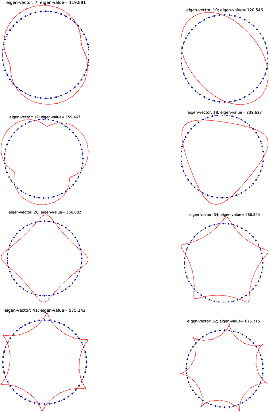
Figure 6. Some of the eigenvalues and the corresponding eigenvectors of the symmetric BEM matrix A represented by the deformed shapes for the circular body.

In Figure 7 (left) it is shown how the theoretically zero eigenvalues associated to rigid body translations are approximated by the two equal and small (possible negative) eigenvalues of the symmetric and non-symmetric BEM matrices A and $\tilde{\text{A}}$, respectively, for a refinement of the boundary element mesh. The absolute values of the numerically computed eigenvalues are plotted in logarithmic scale. These eigenvalues are negative for the symmetric matrix A. Recall that the number of nodes is one half of the number of DOFs. We may observe that these two small eigenvalues are numerically zero regardless discretization in the case of the non-symmetric matrix $\tilde{\text{A}}$. Thus, the symmetric matrix A describes the rigid body motions only approximately (an approximation which is improved with a mesh refinement), while in the case of the non-symmetric matrix $\tilde{\text{A}}$ these rigid body motions are well represented. Finally, in Figure 7 (right) the largest and smallest positive eigenvalues for a mesh refinement are plotted, for both matrices A and $\tilde{\text{A}}$, a very good agreement being observed.

FIGURE 7

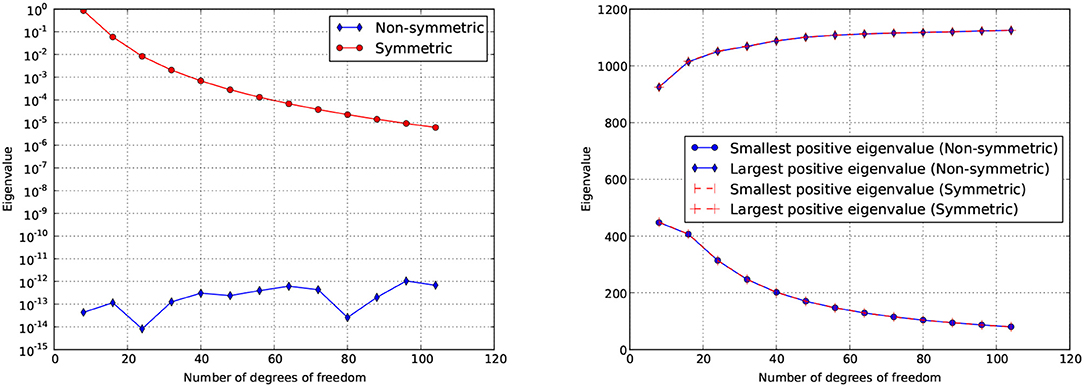
Figure 7. Left: Absolute values of the two equal and small eigenvalues (associated to rigid body translations) of the BEM matrices A and $\tilde{\text{A}}$ for a mesh refinement. Right: The largest and smallest positive eigenvalues of A and $\tilde{\text{A}}$ for a mesh refinement.

In order to numerically study the influence of the application of A instead of $\tilde{\text{A}}$ in BEM calculations, we present the following trivial example whose solution is a rigid body translation. A quadrangular domain is considered with zero tractions on the right and left sides, thus they belong to Γ_N. On the upper side, which belongs to Γ_D, positive normal displacements (in the outward normal direction) are prescribed together with zero horizontal displacements. The bottom side is in frictionless contact with an obstacle, thus it belongs to Γ_C. This problem is quite trivial, since the solution is a rigid body translation in the vertical direction with zero tractions along the whole boundary of the domain. Recall, that in the present computational implementation, both displacements and tractions along the bottom side are considered as unknowns. Figure 8 (left) shows that numerically zero horizontal displacements are obtained, and similarly Figure 8 (right) shows that the vertical displacements accurately represent the rigid body translation by applying the method M1, and also by applying the method M2 where however the non-symmetric matrix $\tilde{\text{A}}$ is used. On the other hand, when the symmetric matrix A is used in the method M2, both results for horizontal and vertical displacements are not so accurate although they improve with the mesh refinement. The main difference from the exact solution is observed near the corners where Γ_C intersects with Γ_N.

FIGURE 8

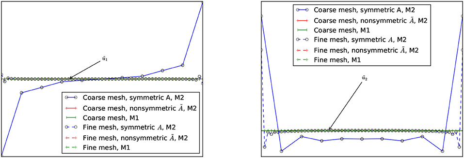
Figure 8. Numerical results along the contact zone, for the trivial contact problem whose solution is a vertical rigid body translation. Left: Horizontal displacements, ũ₁ represents the exact zero horizontal displacement. Right: Vertical displacements, ũ₂ represents the exact vertical displacement.

11. Numerical Examples

A numerical implementation of EC-BEM for both cases of contact was accomplished using an in-house BEM software (Panagiotopoulos, 2017) developed, mainly by the first author, in Java programming language. Linear continuous elements with two nodes are used for the analysis of several examples assuming plane strain conditions. The results obtained by this code are compared with the results obtained by 2D BEM codes developed previously by Blázquez et al. (1998a,b, 2006), and Graciani et al. (2005) in which standard techniques of BEM for contact problems essentially based on the so-called displacement and load scaling techniques (recently also referred to as Sequential Linear Analysis, SLA) (París and Blázquez, 1994) are deployed, as well as by the commercial FEM code ANSYS.

The energetic implementation of the first case of contact described, the Signorini contact, is tested in section 11.1 by solving two problems: one of them with receding contact, in section 11.1.1, and another with advancing contact in section 11.1.2. The case of adhesive unilateral contact is tested in section 11.2 with a similar problem to that used as example of receding contact to test the numerical solution of the Signorini contact problem.

11.1. Numerical Examples to Test the Signorini Contact Implementation

11.1.1. A Case of Receding Signorini Contact

The first problem studied is shown in Figure 9. The geometry is composed by two rectangular solids Ω₁ and Ω₂ in frictionless contact. The shorter rectangle Ω₁, located below, has dimensions (L₇ + L₈ + L₉) × h₁, see Table 3 for lenght values. Vertical and horizontal displacements are restrained, respectively, along a horizontal segment of length L₁ at the lower edge and the lower-left corner of the rectangle. A larger rectangle Ω₂ with dimensions $\sum _{i=1}^6(L_i)\times h_2$ is located at the top. Its vertical and horizontal displacements are restrained, respectively, along an horizontal segment at the lower edge and the upper-right corner. In addition, a uniform vertical displacement u_D is imposed along a segment with dimension L₃ at the upper edge of this rectangle. A segment of length L₈ along the common edge of both solids is defined as potential contact zone, while L₇ and L₉ are assumed to be traction free zones, since separation of the solids is expected, thus, no interpenetration of solids happens along L₇ and L₉. The material of both solids is assumed to be linear elastic and isotropic with properties of aluminum shown in Table 3.

TABLE 3

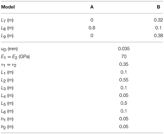
Table 3. Geometry, elastic properties and the imposed displacements.

FIGURE 9

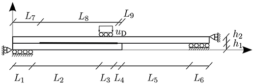
Figure 9. Representation of the receding problem studied: Two beams in contact, Ω₁ and Ω₂, subjected to bending.

In the case of the BEM models presented below, the mesh used is set by the number of elements n_i with i = 1, 2, …, 9 corresponding to the segment of length L_i and n_h1 and n_h2 corresponding to the segments with lengths h₁ and h₂ respectively. Element length is constant along each segment. In the case of the FEM model, solids are meshed in such a way that the nodes along their edges coincide with those in BEM models. Values for the different meshes used here are presented in Table 4.

TABLE 4

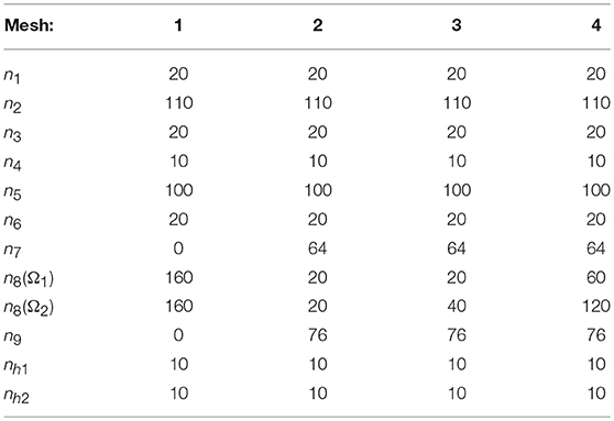
Table 4. Values for the variables n_i.

Along the potential contact zone defined between both solids, two distinct types of contact are considered: (a) unilateral frictionless Signorini contact analyzed in this section, as well as (b) adhesive unilateral frictionless contact shown in section 11.2.

Firstly, computation is carried out taking the model A with the mesh 1 (see Tables 3, 4 respectively). The boundary of the domain Ω₁ is discretized by 340 elements, and that of Ω₂ by 580 elements. The EC-BEM computation works with 160 interface elements along the segment denoted as L₈, requiring the optimization of a quadratic problem of 322 DOFs. Note that n₈ in Table 4 is the same for both solids, so the mesh along the potential contact zone is conforming.

The model is solved by applying the above algorithm. Figure 10 shows the deformed shape, with the scale factor of 500, predicted by the EC-BEM. Note that the potential contact zone is divided into three regions: two segments at both extremes of the initial contact zone where both solids are separated and an active contact zone in the central segment.

FIGURE 10

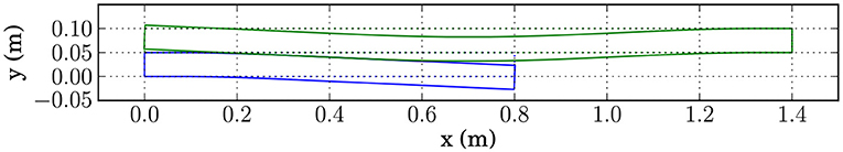
Figure 10. Deformed shape for example A with Signorini contact, with the scale factor of 500.

The numerical results along the potential contact zone are of most interest. Figure 11 shows the normal tractions and relative normal displacements along this boundary part. The central region has compressive tractions and null opening, as expected. On the contrary, normal tractions are almost zero along the regions with a positive relative normal displacement. It is interesting to recall that, in any iteration, during the minimization in the EC-BEM procedure the initial potential contact zone is assumed as a Dirichlet boundary part. According to this, the simultaneity between compressive tractions and null opening or null tractions and positive opening is not explicitly imposed by the algorithm used, as in most contact algorithms. However, the results obtained show that these conditions are well predicted by the energy optimization procedure.

FIGURE 11

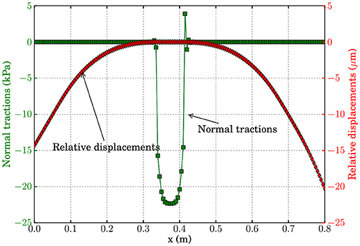
Figure 11. Normal tractions and the relative normal displacements computed along the potential contact zone by the algorithm EC-BEM, for both domains Ω₁ and Ω₂.

Results from the EC-BEM algorithm described here are compared in Figure 12 with the results computed for the same problem with a classic point method algorithm implemented in BEM and the code ANSYS using an Augmented Lagrange algorithm. Note that the agreement between the predictions is accurate in spite of the strong qualitative difference between the different algorithms. The most significant difference is the presence of fictitious oscillations predicted by the EC-BEM at the extremes of contact zone, which do not appear in other numerical results. Also in Figure 12, a second solution obtained by the EC-BEM algorithm and a finer mesh (mesh 2 in Table 4), where additionally a reduced potential contact zone (model B) was assumed, is shown. As can be seen there, the oscillations are reduced, together with the maximum values of the fictitious tensional tractions.

FIGURE 12

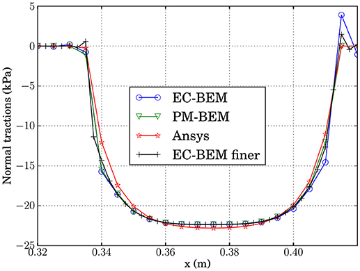
Figure 12. Comparison of tractions computed along the contact zone by the algorithm described here (EC-BEM) and the point method with BEM (PM-BEM) and the FEM code ANSYS using an Augmented Lagrange algorithm. The EC-BEM solution corresponds to model A with Mesh 1, while a finer one also included here, for model B with Mesh 2 (see Tables 3, 4, respectively).

Previous results were obtained using conforming meshes along the potential contact zone. Results obtained with non-conforming meshes are presented in the following. However, strategies presented here for non-conforming meshes are very simple, more advanced formulations may be combined with the present framework for contact problems using energetic principles.

In order to evaluate the influence of a non-conforming mesh on the results obtained by the present algorithm, a computation with the model B and the mesh 3 (see Tables 3, 4 respectively) is carried out. Mesh 3 as well as mesh 4, which have a reduced potential contact zone given by L₈, are defined in view of results of the previous analysis. The number of elements along the potential contact zone of Ω₂ (top) is twice that of Ω₁ (bottom).

As can be seen in Figure 13-top, the normal tractions along the contact boundary of Ω₂, which is the one with finer mesh, present some oscillation around the smooth solution of tractions of Ω₁. This behavior does not depend on the choice of main and secondary domain, a distinction which actually is just auxiliary. Note that, this oscillatory behavior reduces with mesh refinement. In order to observe the reduction of these oscillation, a finer mesh, at the contact boundaries, is employed (mesh 4 in Table 4), maintaining the ratio of number of elements at both sides of the contact zone. Figure 13-bottom shows the comparison of tractions along the boundary of Ω₂ for the coarser and finer mesh. Note that these oscillations are slightly reduced.

FIGURE 13

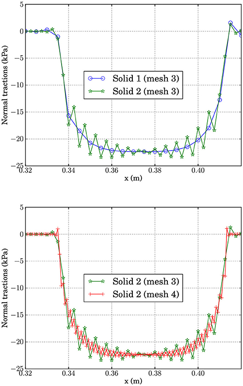
Figure 13. Normal tractions computed along the potential contact zone by EC-BEM, for both domains and for two non-conforming Meshes 3 and 4 of Table 4, with u_D = 0.035 mm.

11.1.2. A Case of Advancing Signorini Contact

The indentation of a half cylinder against an elastic foundation is considered. This is an advancing contact problem as the length of the contact zone depends on the value of the prescribed loading. The problem geometry, shown in Figure 14, is composed by a rectangle with dimensions L₁×h₁ and a half circle with radius h₂. The potential contact zone is defined by the length L₂ and the angle ϕ for the rectangle and the circle respectively. Vertical u_D and null horizontal displacements are imposed along the whole straight edge of the half circle.

FIGURE 14

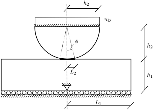
Figure 14. A half elastic cylinder on an elastic rectangle.

Linear elastic and isotropic behavior is assumed for both solids, values of Young's moduli E and Poisson's ratios ν being given in Table 5, where also the geometrical dimensions can be found. The number of elements along each boundary part are detailed in Table 6. Frictionless Signorini contact is considered on the potential contact zone. Due to the fact that this is an advancing contact problem, we are interested in tracking the evolution of the load, which is a non-linear function of the prescribed displacements. In the numerical solution the vertical displacement is introduced by increasing 10 times this displacement in a monotonic way leading to the value u_D shown in Table 5 at the step 10.

TABLE 5

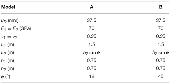
Table 5. Geometry, elastic properties and imposed displacements.

TABLE 6

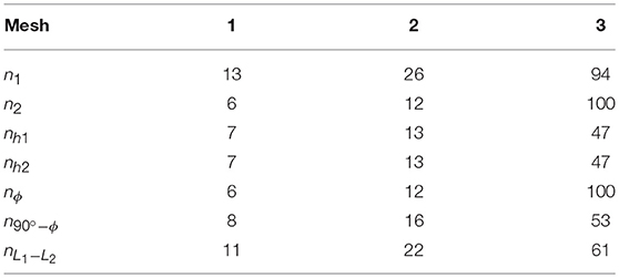
Table 6. Values for the variables n_i defining the different meshes.

The problem is solved using the EC-BEM code described above with the mesh 1 (see Table 6), where n₁, n₂, n_h1 and n_ϕ correspond to the number of elements on the boundary part defined by L₁, L₂, h1 and ϕ respectively. $n_{90^{°}-\varphi }$ is the number of elements along the arc of the half cylinder which is not a potential contact zone and n_L1−L2 is the number of elements at the two parts of the upper edge of the rectangle which are not potential contact zones.

The deformed shape predicted by this code is represented in Figure 15. Consequently, as expected, the vertical displacement imposed on the half circle results in its indentation onto the rectangle. A part of the potential contact zone is in active contact.

FIGURE 15

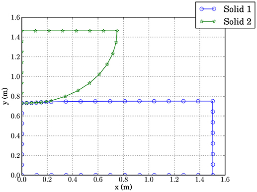
Figure 15. Deformed shape predicted by EC-BEM for Mesh 1 of Table 6.

In a similar way to the example described in section 11.1.1 and for comparison purposes, the problem is solved by the BEM code implementing a classic algorithm of contact by Blázquez et al. (1998a, 2006). The results of the deformed shape around the contact zone for both meshes in Table 6 are represented in Figure 16. Results obtained by the codes using different meshes (see Table 6) and distinct lengths of the potential contact zone (see Table 5). The aim of this figure is to compare both algorithms, and, for that reason, results obtained with the same mesh are grouped. Macroscopically both solutions for EC-BEM and PM-BEM show a very good agreement. However, it is interesting to see in the detailed plot of solutions for mesh 1, plotted in Figure 17, that results for EC-BEM, even for this coarse mesh, show a very good agreement with the Reference solution.

FIGURE 16

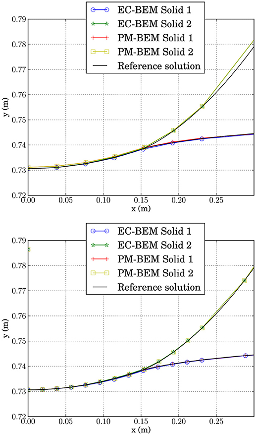
Figure 16. Comparison of the deformed boundaries around the contact zone predicted by EC-BEM, for two different meshes (Mesh 1 and 2 of Table 6 in the top and bottom plot, respectively) with the Reference solution by PM-BEM (using Mesh 3 of Table 6).

FIGURE 17

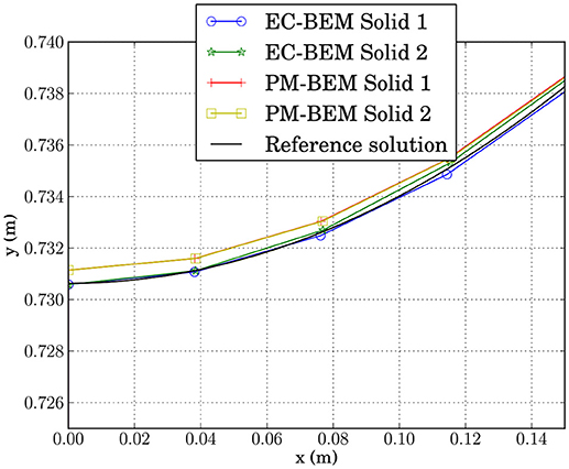
Figure 17. Detailed comparison of the deformed boundaries around the contact zone predicted by EC-BEM and PM-BEM for coarse meshes (Meshes 1 and 2 of Table 6) together with the Reference solution by PM-BEM (using Mesh 3 of Table 6).

A comparison of tractions along the potential contact zone predicted by EC-BEM, PM-BEM and the reference solution is represented in Figure 18. In this figure, unlike those described previously, results are grouped by the method, in order to evaluate the influence of the mesh on the results for each method. Notice that both codes present more accurate results for finer meshes, thus confirming the expected solution convergence with mesh refinement.

FIGURE 18

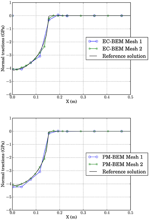
Figure 18. Comparison of the normal tractions computed by EC-BEM and PM-BEM along the interface for different meshes.

The resultant force along the upper part Γ_D of the half cylinder can be estimated from the results of tractions predicted by both methods. In particular, we focus on the vertical component F_y of this force because it is the only one which produces work since horizontal displacements are zero by the boundary conditions. This value is calculated by the integration of stresses over Γ_D,

$\begin{array}{rc}{F}_y={\displaystyle \underset{{\Gamma }_{\text{D}}}{\int }}{\sigma }_{yy}\mathrm{\text{d}}x& (48)\end{array}$

where σ_yy represent the normal tractions at the nodes. The integral is calculated by a standard quadrature.

The values of the resultant force F_y, calculated for the 10 steps by both codes, are represented in Figure 19 as a function of the vertical displacement imposed. Both codes predict that stiffness is increasing with the vertical displacement, as typical for the Hertz contact problems. The reason is that the contact zone between both solids is enlarging, with a consequence that the global system becomes stiffer.

FIGURE 19

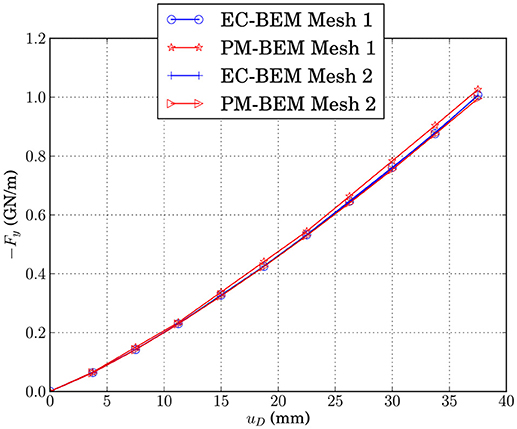
Figure 19. Force F_y predicted by both methods as a function of the imposed vertical displacement u_D.

11.2. Numerical Examples to Test the Adhesive Contact Implementation

This section aims to compare the results obtained by the energetic approach and commercial FEM code (ANSYS, 2010) in the case of the elastic contact described in section 2. To this effect, the problem of receding contact studied above is solved again, this time with the contact conditions of the adhesive elastic contact.

The problem represented in Figure 9 is studied with the properties of model A, see Table 3, and the mesh 1, see Table 4. The stiffness parameters, assumed for this example, are κ_n = 150 GPa/m and κ_t = 0.

Results from the EC-BEM computations for displacements and tractions along the boundary between both solids are presented in Figure 20. As expected, zones with tensions correspond to positive relative displacements (external zones for example) and zones with compressions correspond to vanishing relative displacements (zones adjacent to the previous ones). In this case, a strongly complex zone is predicted at the center of the boundary, which will be studied below.

FIGURE 20

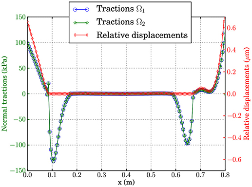
Figure 20. Normal tractions and normal relative displacements along the potential contact zone in the example of Figure 9 with the adhesive elastic contact computed by EC-BEM, and with u_D = 0.035 mm.

For comparison purposes, the problem is solved using the FEM code (ANSYS, 2010) setting the contact properties in the following way:

• Contact behavior: No separation (always)

• Contact: Surface to surface

• Contact algorithm: Penalty method

• Contact detection: At nodal points (normal from contact nodes)

• Opening contact stiffness (KFOP): κ_n

Results for tractions in the solids obtained by ANSYS and the EC-BEM code are compared in Figure 21. In the upper figure we can observe that the agreement along the four zones described above is accurate. It is interesting to focus on the zone in the middle of the boundary where tractions looks like vanishing at the scale of the upper figure. Lower figure shows the complexity of this zone, which is composed by two lateral regions where both solids are separated and a central region where both solids are under contact (compression). The agreement between both results is reasonable in spite of the very small scale compared to the tractions obtained on the whole boundary.

FIGURE 21

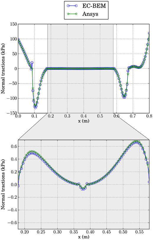
Figure 21. Comparison of the normal tractions computed by EC-BEM and ANSYS for the adhesive elastic contact, with u_D = 0.035 mm.

A subsequent analysis is carried out by multiplying the displacement u_D by 100 without modifying any other parameters in both codes. In this case, the results from the energetic approach presented here remain qualitatively similar, whereas the results from ANSYS present some problems to match the complex central zone. To the knowledge of authors, this could be solved by modifying some of the values of the key-options which configure the contact algorithm of ANSYS. This shows the robustness of the energetic approach compared to other contact algorithms, where convergence depends on the value of certain non-physical parameters of the numerical model.

12. Concluding Remarks

A novel approach for contact problems of elastic bodies was presented. This method is based on the energy principles expressed by boundary integrals. The solution of contact problems is obtained by the minimization of the total potential energy. Appropriate algorithms to solve the quadratic problems were presented. The cases of conforming as well as non-conforming meshes for contact zone were addressed.

Numerical examples, showing the suitability of the present framework to solve typical contact problems were examined, and also successfully compared to other well established BEM methodologies as well as a commercial FEM code.

The proposed framework can be easily incorporated to existing BEM or FEM codes. Possible extension to the case of elastodynamics, where instead of the principle of virtual work we may use the principle of virtual power in order to compute the total energy (kinetic plus elastic), using only boundary values, of tractions and velocities, is possible. For this it might be convenient to utilize a formulation such as that introduced in Panagiotopoulos and Manolis (2010, 2011).

Finally, the present framework is found to be very useful in the case where also dissipative mechanisms exist on the boundaries or common interfaces of elastic bodies. In such cases we may apply energetic approaches to solve the corresponding non-linear problems as was shown in previous publications by some of the present authors (e.g., Panagiotopoulos et al., 2013).

Author Contributions

All authors listed have made a substantial, direct and intellectual contribution to the work, and approved it for publication.

Funding

The authors acknowledgethe support by the Junta de Andalucía and European Social Fund (Proyecto de Excelencia TEP-4051), the Spanish Ministry of Science and Innovation (Project MAT2009-14022), the Spanish Ministry of Economy and Competitiveness and European Regional Development Fund (Projects MAT2012-37387 and MAT2015-71036-P), and Spanish Ministry of Education (FPU grant AP2009-3968). Furthermore, CP acknowledges the financial support of the Stavros Niarchos Foundation within the framework of the project ARCHERS (Advancing Young Researchers' Human Capital in Cutting Edge Technologies in the Preservation of Cultural Heritage and the Tackling of Societal Challenges).

Conflict of Interest Statement

The authors declare that the research was conducted in the absence of any commercial or financial relationships that could be construed as a potential conflict of interest.

Acknowledgments

The authors would like to express their gratitude to Prof. Tomáš Roubíček of the Charles University of Prague, as well as to Dr. Roman Vodička from the Technical University of Košice, for fruitful discussions.

References

Aliabadi, M. H. (2002). The Boundary Element Method: Applications in Solids and Structures. Chichester, UK: Wiley.

Google Scholar

ANSYS (2010). ANSYS Mechanical APDL Contact Technology Guide Release 13.0. Canonsburg, PA: Ansys, Inc.

Antes, H., and Panagiotopoulos, P. D. (1992). The Boundary Integral Approach to Static and Dynamics Contact Problems. Equality and Inequality Methods, Vol. 108 of International Series of Numerical Mathematics. Basel: Birkhauser Verlag.

Aour, B., Rahmani, O., and Nait-Abdelaziz, M. (2007). A coupled FEM/BEM approach and its accuracy for solving crack problems in fracture mechanics. Int. J. Solids Struct. 44, 2523–2539. doi: 10.1016/j.ijsolstr.2006.08.001

CrossRef Full Text | Google Scholar

Axelsson, O. (1980). Conjugate gradient type methods for unsymmetric and inconsistent systems of linear equations. Linear Algebra Applic. 29, 1–16. doi: 10.1016/0024-3795(80)90226-8

CrossRef Full Text | Google Scholar

Blázquez, A., Mantič, V., and París, F. (2006). Application of BEM to generalized plane problems for anisotropic elastic materials in presence of contact. Eng. Anal. Bound. Elements 30, 489–502. doi: 10.1016/j.enganabound.2005.07.006

CrossRef Full Text | Google Scholar

Blázquez, A., and París, F. (2009). On the necessity of non-conforming algorithms for “small displacement” contact problems and conforming discretizations by BEM. Eng. Anal. Bound. Elements 33, 184–190. doi: 10.1016/j.enganabound.2008.05.003

CrossRef Full Text | Google Scholar

Blázquez, A., París, F., and Cañas, J. (1998a). Interpretation of the problems found in applying contact conditions in node-to-point schemes with boundary element non-conforming discretizations. Eng. Anal. Bound. Elements 21, 361–375. doi: 10.1016/S0955-7997(98)00024-1

CrossRef Full Text | Google Scholar

Blázquez, A., París, F., and Mantič, V. (1998b). BEM solution of two-dimensional contact problems by weak application of contact conditions with non-conforming discretizations. Int. J. Solids Struct. 35, 3259–3278. doi: 10.1016/S0020-7683(98)00016-X

CrossRef Full Text | Google Scholar

de Paula, F. A., and Telles, J. (1989). A comparison between point collocation and Galerkin for stiffness matrices obtained by boundary elements. Eng. Anal. Bound. Elements 6, 123–128. doi: 10.1016/0955-7997(89)90025-8

CrossRef Full Text | Google Scholar

Dostál, Z. (2009). Optimal Quadratic Programming Algorithms: With Applications to Variational Inequalities, Vol. 23 of Springer Optimization and Its Applications. New York, NY: Springer Science+Business Media.

Google Scholar

Eck, C., Jarušek, J., and Krbec, M. (2005). Unilateral Contact Problems. Variational Methods and Existence Theorems. Boca Raton, FL: Chapman & Hall; CRC; Taylor & Francis Group.

Google Scholar

Fichera, G. (1964). Problemi elastostatici con vincoli unilaterali: il problema di signorini con ambigue condizioni al contorno. Mem. Accad. Naz. Lincei VIII, 91–140.

Google Scholar

Gakwaya, A., Lambert, D., and Cardou, A. (1992). A boundary element and mathematical programming approach for frictional contact problems. Comput. Struct. 42, 341–353. doi: 10.1016/0045-7949(92)90030-4

CrossRef Full Text | Google Scholar

Graciani, E., Mantič, V., París, F., and Blázquez, A. (2005). Weak formulation of axi-symmetric frictionless contact problems with boundary elements. application to interface cracks. Comput. Struct. 83, 836–855. doi: 10.1016/j.compstruc.2004.09.011

CrossRef Full Text | Google Scholar

Graciani, E., Mantič, V., París, F., and Varna, J. (2009). Numerical analysis of debond propagation in the single fibre fragmentation test. Compos. Sci. Technol. 69, 2514–2520. doi: 10.1016/j.compscitech.2009.07.006

CrossRef Full Text | Google Scholar

Gurtin, M. E. (1972). The Linear Theory of Elasticity, Vol. VIa/2 of Handbuch der Physik. Berling: Springer-Verlag.

Google Scholar

Hartmann, F. (1981). The derivation of stiffness matrices from integral equations. Appl. Math. Model. 5, 355–365. doi: 10.1016/S0307-904X(81)80058-3

CrossRef Full Text | Google Scholar

Hertz, H. (1896). Miscellaneous Papers on the Contact of Elastic Solids. Trans. D. E. Jones (London: McMillan).

Hestenes, M. R., and Stiefel, E. (1952). Methods of conjugate gradients for solving linear systems. J. Res. Natl. Bur. Stand. 49, 409–436. doi: 10.6028/jres.049.044

CrossRef Full Text | Google Scholar

Johnson, K. L. (1985). Contact Mechanics. Cambridge: Cambridge University Press.

Google Scholar

Kalker, J., and Randen, Y. V. (1972). A minimum principle for frictionless elastic contact with application to non-Hertzian half-space contact problems. J. Eng. Math. 6, 193–206. doi: 10.1007/BF01535102

CrossRef Full Text | Google Scholar

Katsikadelis, J., and Kokkinos, F. (1993). Analysis of composite shear walls with interface separation, friction and slip using bem. Int. J. Solids Struct. 30, 1825–1848. doi: 10.1016/0020-7683(93)90236-Z

CrossRef Full Text | Google Scholar

Lazaridis, P. P., and Panagiotopoulos, P. D. (1987). Boundary variational “principles” for inequality structural analysis problems and numerical applications. Comput. Struct. 25, 35–49. doi: 10.1016/0045-7949(87)90216-1

CrossRef Full Text | Google Scholar

Mantič, V. (1993). A new formula for the C-matrix in the Somigliana identity. J. Elastic. 33, 191–201. doi: 10.1007/BF00043247

CrossRef Full Text | Google Scholar

Méchain-Renaud, C., and Cimetière, A. (2000). Influence of a curvature discontinuity on the pressure distribution in two-dimensional frictionless contact problems. Int. J. Eng. Sci. 38, 197–205. doi: 10.1016/S0020-7225(99)00018-X

CrossRef Full Text | Google Scholar

Panagiotopoulos, C. G. (2017). Symplegma: Java Components for Computational Mechanics and Numerical Modelling. Available online at: http://symplegma.org/

Panagiotopoulos, C. G., and Manolis, G. D. (2010). Velocity-based reciprocal theorems in elastodynamics and BIEM implementation issues. Arch. Appl. Mechan. 80, 1429–1447. doi: 10.1007/s00419-009-0376-0

CrossRef Full Text | Google Scholar

Panagiotopoulos, C. G., and Manolis, G. D. (2011). Three-dimensional BEM for transient elastodynamics based on the velocity reciprocal theorem. Eng. Anal. Bound. Elements 35, 507–516. doi: 10.1016/j.enganabound.2010.09.002

CrossRef Full Text | Google Scholar

Panagiotopoulos, C. G., Mantič, V., and Roubíček, T. (2013). BEM solution of delamination problems using an interface damage and plasticity model. Computat. Mechan. 51, 505–521. doi: 10.1007/s00466-012-0826-3

CrossRef Full Text | Google Scholar

Panagiotopoulos, P. D., and Lazaridis, P. P. (1987). Boundary minimum principles for the unilateral contact problems. Int. J. Solids Struct. 23, 1465–1484. doi: 10.1016/0020-7683(87)90064-3

CrossRef Full Text | Google Scholar

París, F., and Blázquez, A. (1994). On the displacement and load scaling techniques in contact problems using bem. Bound. Elements Commun. 5, 15–17.

Google Scholar

París, F., Blázquez, A., and Cañas, J. (1995). Contact problems with nonconforming discretizations using boundary element method. Comput. Struct. 57, 829–839. doi: 10.1016/0045-7949(95)92007-5

CrossRef Full Text | Google Scholar

París, F. and Cañas, J. (1997). Boundary Element Method, Fundamentals and Applications. Oxford: Oxford University Press.

Google Scholar

París, F., and Garrido, J. A. (1989). An incremental procedure for friction contact problems with the boundary element method. Eng. Anal. Bound. Elements 6, 202–213. doi: 10.1016/0955-7997(89)90019-2

CrossRef Full Text | Google Scholar

Renaud, C., and Feng, Z.-Q. (2003). BEM and FEM analysis of Signorini contact problems with friction. Comput. Mechan. 31, 390–399. doi: 10.1007/s00466-003-0441-4

CrossRef Full Text | Google Scholar

Roubíček, T., Mantič, V., and Panagiotopoulos, C. G. (2013). A quasistatic mixed-mode delamination model. Disc. Cont. Dynam. Syst. S 6, 591–610. doi: 10.3934/dcdss.2013.6.591

CrossRef Full Text | Google Scholar

Saad, Y. and Schultz, M. H. (1985). Conjugate gradient-like algorithms for solving nonsymmetric linear systems. Math. Comput. 44, 417–424. doi: 10.1090/S0025-5718-1985-0777273-9

CrossRef Full Text | Google Scholar

Signorini, A. (1959). Questioni di elasticità non linearizzata e semilinearizzata. Rendiconti di Matematica e delle sue Applicazioni 18, 95–139.

Google Scholar

Stavroulakis, G. E., and Antes, H. (1997). Nondestructive elastostatic identification of unilateral cracks through BEM and networks. Comput. Mechan. 20, 439–451. doi: 10.1007/s004660050264

CrossRef Full Text | Google Scholar

Tullberg, O., and Bolteus, L. (1982). “A critical study of different boundary element stiffness matrices,” in Boundary Element Methods in Engineering, ed C. A. Brebbia (Berling: Springer–Verlag), 621–635.

Google Scholar

Vodička, R. (2000). The first and the second–kind boundary integral equation systems for solution of frictionless contact problems. Eng. Anal. Bound. Elements 24, 407–426. doi: 10.1016/S0955-7997(00)00012-6

CrossRef Full Text | Google Scholar

Wriggers, P. (2006). Computational Contact Mechanics, 2nd Edn. Berling: Springer.

Google Scholar

Wriggers, P., and Panagiotopoulos, P. D. (1972). New Developments in Contact Problems, Vol. 384 of CISM courses and lectures. NewYork, NY: Springer Wien.

Google Scholar

Yastrebov, V. A. (2013). Numerical Methods in Contact Mechanics. London, UK: ISTE Ltd and Wiley.

Google Scholar

Zhou, C., Byrd, R. H., Lu, P., and Nocedal, J. (1997). Algorithm 778: L-BFGS-B: Fortran subroutines for large-scale bound-constrained optimization. ACM Trans. Math. Soft. 23, 550–560. doi: 10.1145/279232.279236

CrossRef Full Text | Google Scholar