- Department of Business and Economics, University of Cagliari, Cagliari, Italy
We develop a general framework to apply the Kelly criterion to the stock market data, and consequently, to portfolio optimization. Under few conditions, using Monte Carlo simulations with different scenarios we prove that the Kelly criterion beats any other approach in many aspects. In particular, it maximizes the expected growth rate and the median of the terminal wealth. We also show that, under a normal distribution of returns, the Kelly criterion has the best performance in the long run. Next, we optimize a portfolio with the Kelly criterion with no leverage and no short selling conditions and show that this portfolio lays in the mean-variance efficient frontier and has higher expected return and higher variance, although it is less diversified, respect to the tangent portfolio optimized under the Markowitz approach. Finally, we implement a dynamic strategy applied on the European stock market data and compare the results between the tangent and the optimal Kelly portfolios. In a dynamic setting, the rolling Kelly portfolio outperforms competitors particularly in the case of rebalanced portfolios optimized with a 2-years window width.
1. Introduction
When an investor allocates his money in the market, what he aims to is making much money as possible at the lowest level of risk. In literature, many researchers have come up with different solutions for the investor problem. One of the most famous is proposed by Markowitz [1]. An alternative approach is the Kelly criterion. It derives from the work of John Larry Kelly Jr, who was a researcher at Bell Labs. In his seminal paper [2], Kelly utilizes the logarithmic function for the solution of investment problems. He demonstrates that the logarithmic function maximizes the long period growth rate, but it is myopic, as it maximizes the capital in the current interval only, regardless of past or future information. Basically, Kelly defines how much fraction it is best to invest in a single bet and consequently in a series of bets when the probability and the net outcomes are known. The Kelly criterion not only works at its finest when we know the actual probability and net income of our bets, but it is also superior to any essentially different strategy when we just know the probability distribution of the returns.
The main purpose of this paper is to show the theoretical framework of the Kelly criterion and to demonstrate its good and bad properties through the implementation of the method under different conditions. In particular, we consider the performance of portfolios specified under the Kelly criterion for the stock market, and implement an optimization method that considers the Kelly criterion to define a portfolio composed of a large set of European financial assets listed in the EuroStoxx50 and observed from 2007 to 2019. We compare the results obtained for the portfolio based on the Kelly criterion, hereafter the Kelly portfolio, with those deriving from portfolios optimized under the Mean-Variance approach. First, an in-sample analysis is performed by expanding the work of Kim and Shin [3]: the correlation between assets is considered and a continuous probability distribution for the assets' returns is specified. Next, a out-of-sample analysis is performed exploiting the work of Estrada [4] but using an alternative approach to compute the Kelly fractions and implementing a more active rebalancing strategy based on the readjustment of the portfolio weights at the end of each time period. Empirical results show that Kelly portfolios are more risky but, if certain conditions are met, they bring a much higher reward in terms of final wealth, whilst the Tangent portfolio cannot reach its goal, leading to a lower Sharpe ratio respect to the Kelly portfolio. A sensitivity analysis demonstrates that the choice of the period length to compute both the variance-covariance matrix and the expected returns, and the choice of the frequency of rebalancing, are fundamental for reaching the highest returns. In particular, a short length of the window width using in a rolling portfolio optimization framework guarantees that the Kelly portfolio outperforms competitors w.r.t. the out of sample annual growth rate and despite the frequency of rebalancing.
The remainder of the paper is organized as follows. Section 2 explains briefly the theoretical background of the Kelly criterion and its critiques. Section 3 describes the method analytically and introduces an ad-hoc defined optimization method for the maximization of the expected growth rate of a portfolio based on the Kelly criterion. An extended simulation study investigating about the effectiveness of the Kelly criterion and its properties is presented in section 4. Section 5 shows the results obtained from the application of the Kelly criterion on real data from European stocks and, in particular, to both the static and dynamic portfolio optimization case. Section 6 ends the paper with some concluding remarks.
2. Materials and Methods
2.1. Background
Markowitz portfolio optimization achieves simplicity in the mean–variance model by focusing on the economic trade-off between risk and return in a single-period case. However, many investors make portfolio decisions in a multiperiod case where portfolios are rebalanced periodically. For these investors, Latané [5] recommends an alternative framework, the geometric mean or growth optimal portfolio model, arguing that the maximum geometric mean strategy almost surely leads to greater wealth in the long run than any significantly different portfolio strategy. This result follows from similar conclusions of John Kelly [2] in the context of information theory. He outlines how a receiver of a noisy signal containing information on the outcome of a game can use that information to his advantage in gambling. Next, gamblers and investors have used the criterion formalized by Kelly that became known as the “Kelly criterion for investing and risk management.” Breiman [6] provides rigorous mathematical proofs of the Kelly criterion. He defines and demonstrates all its properties as well as that under some conditions it can be considered as the best strategy to use. But much of what we know about the use of the Kelly criterion comes from the work of Edward Thorp [7, 8], which is the first gambler who uses the Kelly criterion to beat the Las Vegas casinos playing black jack. Next, he focuses the attention on the stock market and he became one of the most efficient trader on Wall Street. Thorp shows how to use the Kelly criterion as a portfolio optimization method based on an unconstrained optimal solution, as well as how to use it to decide which position is better to take w.r.t. different types of financial assets.
Unfortunately, although for discrete probability distributions the optimal solution can be found analytically, for assets that have a continuous probability distribution, such as portfolios, the solution of the optimization problem is derived from a second order Taylor approximation under the assumption of a Gaussian distribution of returns. As for the Taylor approximation, Nekrasov [9] introduces an algorithm that considers the approximation used to define the optimal portfolio computed w.r.t. the Thorpe formula. In contrast, Kim and Shin [3] do not make assumptions on the probability distribution of returns and define a ratio between average returns using historical data. They suggest to start from historical stock returns and compute both the probability that a stock price increases and the “average winning and loss ratio.” The latter is computed as the ratio between the average return when a stock price increases and the average return when the stock price decreases. With these inputs, they derive the optimal Kelly ratio. Using this method on data from the Korean stock market, they find that portfolios optimized under the Kelly criterion with no leverage and no short selling have higher returns and higher variance compared to the tangent portfolio optimized under the Markowitz approach. The latter is less diversified but lays on the efficient frontier. Similar results appear in Estrada [4], where it is reported that the Kelly criterion is superior to traditional strategies in terms of long-term growth, and that Kelly portfolios are less diversified and have both an higher expected return and an higher volatility compared to portfolios composed with the goal of maximizing risk-adjusted returns. Likewise, Fama and McBeth [10] demonstrate, using samples of NYSE stocks, that the Kelly portfolios have higher geometric mean return and beta risk than the market portfolios. Finally, MacLean et al. [11] summarize the good and bad properties of a Kelly strategy arguing that: (a) maximizing the expected utility E[log X] asymptotically corresponds to maximize the assets growth rate; (b) under fairly conditions, maximizing E[log X] leads asymptotically to maximize the median of log X; (c) the Kelly gambler never risks ruin. These results are consistent with those showed in Ziemba [12], where it is demonstrated that the expected time required by the Kelly criterion to reach a preassigned goal is, asymptotically as X increases, least with a strategy maximizing E[log X]. Moreover, MacLean et al. [11] also show that, if an investor wishes to bear lower risk trading it off for lower reward, he should use a fractional Kelly strategy. They warn that using the Kelly strategy can lead to bets that may be a large fraction of the current wealth of the investor when the wager is favorable and the risk of loss is very small. In the same line of research, particularly interesting are the theoretical results introduced in Browne and Whitt [13] and in Lo et al. [14]. The first study defines optimal gambling and investment policies using a Bayesian approach for the case the underlying stochastic process has parameters' values that are unobserved random variables, so that the optimal strategy is to bet a fraction of current wealth deriving from a linear function of the posterior mean increments [13]. The second study demonstrates that the optimal behavior of an investor using the Kelly criterion is obtained when she maximizes her absolute wealth in the case of an infinite horizon. In the case that she maximizes her relative wealth, the conditions under which the Kelly criterion is optimal and those under which the investor should deviate from it are identified. In particular, the investor's initial relative wealth plays a critical role and the dominant investor's optimal behavior is different from the minorant investor's optimal behavior [14].
Nowadays many hedge fund managers, including Warren Buffet from Berkshire Hathaway and George Soros, utilize the Kelly criterion in their asset allocation strategies [15]. However, the problem with portfolios composed in accordance with the Kelly criterion is that these portfolios are riskier than other portfolios (e.g., efficient mean-variance portfolios) in the short term. In view of that, Thorp [16] suggests that the logarithmic utility theory deriving from the Kelly criterion has a normative or prescriptive nature, but only for those institutions, groups or individuals whose overriding current objective is maximization of the rate of asset growth. This might be the reason why, as stated before, Kelly portfolios are often used by big hedge fund managers who focus on the long-term growth maximization rather than on the avoidance of short-term losses. To reduce the risk profile of Kelly portfolios, a fractional Kelly approach can be used. It is based on a “investing less than the optimal” strategy. The less-than-optimal investment fraction is easy to determine analytically in the univariate case, whilst for multi-asset portfolio optimization the analytical solution is hard to be found. Davis and Lleo [17] extend the definition of fractional Kelly strategies to the case where the investor's objective is to outperform a benchmark. They theoretically define benchmarked fractional Kelly strategies as efficient portfolios even when asset returns are not lognormally distributed. Peterson [18] demonstrates that the Kelly criterion can be incorporated into standard portfolio optimization models that include a risk function. The risk and return functions are combined into a single objective function using a risk parameter and the optimization is based on a differential evolution algorithm providing optimal returns for the Kelly portfolios that are similar to those obtained from the Markowitz approach. In the same framework, Rising and Wyner [19] derived a fractional Kelly portfolio and showed that it is identical to the full Kelly portfolio optimized on the basis of an estimate of the expected asset return vector, which is statistically shrunken to the risk-less rate. In other words, their approach is based on the consideration that a fractional Kelly investor turns out to be a full Kelly investor who uses shrinkage estimates of the markets' parameters. In contrast, Han et al. [20] shrunk the Kelly portfolio weights directly rather than shrinking the expected return toward the risk-free rate. Their approach is based on the idea of minimizing the expected growth loss of the actual growth based on the plug-in estimates of the true growth rate. Almost at the same time, Hsieh and Barmish [21] claim that, when the optimal Kelly fraction increases, various risk measures become excessively large providing poor drawdown performances whilst the Kelly strategy, although being log-growth optimal, may be too aggressive in the short term. The authors also disagree with the use of the Taylor series to compute the optimal Kelly fraction, arguing that this solution may lead to performances lower than that of the true optimum. Consequently, Busseti et al. [22] add a drawdown risk constraint in the optimization problem specified for a portfolio optimized under the Kelly criterion to lower the risk that this kind of portfolio has, and argue that this new constraint can somehow be seen as a risk-aversion parameter. Osorio [23], instead, argues that stock prices are not log-normally distributed and that both excess kurtosis and skewness cannot be sufficiently captured. Thus, the Kelly fractions under the hypothesis that returns follow a Student t-distribution is derived analytically.
Recently, few researchers are starting to study how the Kelly criterion can be used on option portfolios. Aurell et al. [24] are the first to use the Kelly criterion in order to specify a model to price and hedge derivatives in incomplete markets. Wu and Chung [25] implement an algorithm that seems able to find the most profitable option portfolio using the Kelly criterion. Using data from the Taiwan Stock Exchange Index they demonstrate that trading signals obtained from traditional strategies were not necessary when using the Kelly criterion. Finally, Wu and Hung [26] use the Kelly criterion within a framework where a strategy involving trading on options exercised on the simple index futures is defined. Their strategy is based on some entering signals, such as golden-death cross.
In this paper, we discuss the Kelly criterion and prove its most interesting properties with various Monte Carlo simulations under different scenarios. The Kelly criterion is implemented in a realistic investment situation using data from the European equity market, both for a single asset and a portfolio of securities. The main innovation with respect to previous studies is that, in our settings, portfolios are implemented such that in each period the expected growth rate is maximized despite the length of the period. This is done taking into account the correlation among the assets and the hypothesis of normal distribution of returns. We compare the results with the traditional portfolio optimized under the Mean-Variance approach, that assumes that the investment decisions are solely made with regard to the mean and variance of returns.
2.2. Methods
In this section, we introduce the fundamental concepts of the Kelly criterion for discrete and continuous probability distribution, as well as for both the univariate and multivariate cases.
2.2.1. Discrete Probability
Following Rotando and Thorp [27], we consider a series of favorable bets, where a favorable bet is a bet where the following condition holds
Zn is the final wealth after n trials. An example of a favorable bet might be a biased coin where the winning probability is p > 1/2. Let us imagine that for deciding how much of our capital is allocated to the wager amount we maximize its expected value. Thus, in each trial we invest all of our wealth in the game. The problem with this strategy is that ruin becomes almost sure as the number of trials tends to infinity. In this situation, minimizing the probability of eventual ruin is not desirable as it corresponds to minimizing at the same time the expected average gain.
Starting from the scenario described above, Kelly introduced an alternative strategy that is intermediate between maximizing gain and minimizing the probability of ruin. Let's assume that the condition specified in Equation (1) still holds and we observe a winning probability 1/2 < p ≤ 1 associated to the outcome 1, and a losing probability q = (1−p) associated to the outcome −1. Starting with an initial wealth W0, we suppose to bet a faction f of the initial wealth. After n trials where we win m times, the final wealth is given by:
since
In this framework, the exponential rate of the asset growth per trial is
Kelly chooses to maximize the expected value of the growth rate coefficient G(f), namely
To maximize G(f), we need to derive Equation (2) respect to f:
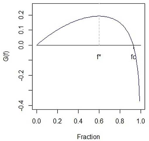
The value of f that maximizes G(f) is f* = p − q. It is also shown that f* is the unique maximum of G(f), since:
Thus, G′(f) is monotone strictly decreasing in [0, 1), whilst G′(0) = p − q > 0 and . Plugging f* = p − q into Equation (2) we obtain
Moreover, since G(0) = 0 and , there is a unique value fc > 0 and 0 < f* < fc < 1, such that G(fc) = 0.
The growth rate function G(f) is represented in Figure 1 w.r.t. different values of the fraction of wealth f.
Breiman [6] and Thorp [7] demonstrate that the final wealth of the player Wn exceed any fixed bound M when 0 < f < fc, but not for a finite number of trials. In contrast, ruin is going to happen almost surely if f > fc. In the case f = fc, the wealth after n trials will oscillate randomly between 0 and +∞. Moreover, the Kelly criterion beats any other strategy over a long period of time and it asymptotically minimizes the time required to reach a certain level of wealth. The criterion is still valid even if the probability changes over the trials. In this case, a subject must choose the optimal in each trial in order to maximize E[log Wn].
2.2.2. Continuous Probability Distribution
To implement the Kelly Criterion for a portfolio of securities, it is necessary to consider the case of continuous probability distributions. Following Thorp [8], let us suppose we have an initial wealth W0 and we want to determine the optimal betting fraction f* to invest each time in a financial asset. The problem is that, unlike in the previous case, for a financial asset there is no finite number of outcomes of a bet, thus we cannot use discrete distributions but we need to refer to continuous distributions. In this case the goal is maximizing
where P(x) is a probability measure for the outcome and f is the fraction of invested capital. We assume a constraint 1 + fx > 0 in order to avoid undefined logarithms. If the outcomes of x are distributed as a symmetric random variable around E(x) = μ with Var(x) = σ2, then:
With this assumption we are simplifying the experiment of investing in the stock market by splitting it into two separate outcomes. If positive, the return per unit of investment is μ + σ, otherwise it is μ − σ. The wealth W can thus be described as
where r is the return obtained on a risk-free asset, such as a treasury bond. Hence, the expected growth rate g(f) is defined as
Next, if the time interval is divided into n sub-intervals of the same length it is possible to consider n independent random variables xi with mean and variance . For each xi, it results
The ratio between the final wealth Wn(f) and the initial wealth W0 is
The expectation of the natural logarithm on both sides of Equation (4) gives g(f), which is represented with a second order Taylor approximation centered in f = 0
and re-scaled w.r.t. n
In Equation (5), U = ±1 is a symmetric Bernoulli random variable and the expansion , when u → 0, yields
Since E(U) = 0 and E(U2) = 1, Equation (6) reduces to
As approaches 0. In this case, Equation (7) results in
The optimal Kelly fraction f is found maximizing g∞(f), i.e., differentiating Equation (8) w.r.t f
Thorp [8] observes that, as n → ∞, the limit value of Wn(f) corresponds to a log normal diffusion process with an underlying security having mean μ and variance σ2. This is a well-known model for securities' prices. Thus, g∞(f) is the instantaneous growth rate of the invested capital characterized by a betting fraction f. Betting the optimal fraction f* leads to a growth rate
Compared to the case of a discrete distribution, the constraint 0 ≤ f < 1 is not required. The additional constraint 1 + fx > 0 required in Equation (3) is also not required. The case f < 0 is now feasible, as it simply requires selling the security short and this strategy could be advantageous when μ < r. The investor who follows this strategy has to adjust his investment “instantaneously.” This conceptualization appears in the option theory and does not prevent the practical application of the model [28].
2.2.3. Implementing Kelly Criterion Portfolios
Beside investing in a single financial asset it is also possible to compose portfolios optimized under the Kelly criterion. In the following we use the term Kelly portfolio to refer to such a kind of portfolio.
Consider a risk-free asset with a portfolio fraction f0 and n risky assets with portfolio fraction f1,…, fn. Let r be the return of the risk-free asset corresponding to the borrowing rate as well as to the rate paid in the case of selling. If Σ = (si,j), with i, j = 1, 2,…, n, is the variance-covariance matrix of assets' returns and is the row vector of the expected returns for the n assets, a Kelly portfolio satisfies
To find the optimal F*, it is necessary to maximize
Equation (11) corresponds to a quadratic maximization problem with an unconstrained solution:
A unique solution of Equation (12) requires the existence of Σ−1. In the case of uncorrelated assets' returns the variance-covariance matrix Σ is diagonal and the optimal fraction, deriving from the Kelly criterion, is
The Kelly portfolios are optimized under the no leverage and no short selling conditions. Applying roughly Equation (12) under these conditions would lead us to consider a unconstrained portfolio. To overcome this situation, we consider the maximization of the expected growth rate g*, under no short and no leverage constraints, as the reference optimization criterion. Notationally, it corresponds to:
where r, F, and M have been defined in Equations (10) and (11), respectively, and is the plug-in estimator of the variance-covariance matrix Σ. The maximization of g* is constrained on portfolio weights fi defined in [0, 1] and such that they sum up to one, that is: to the fully invested capital condition. The optimization criterion specified in Equation (13) is a quadratic maximization problem allowing us to determine the fractions of wealth to be allocated to each single equity.
All the computations presented in the following are performed using the R software for statistical computing [29] installed on a PC equipped with a Intel i9 5.3 GHz processor. In particular, the quadprog [30] library is used to implement the optimization method introduced in section 2.2.3 for Kelly portfolios and the library fPortfolio [31] is used to define portfolio compositions based on the Markowitz method.
2.3. Monte Carlo Simulations
In the previous sections we have described the Kelly criterion and its properties. In the following, we perform some experiments through Monte Carlo simulations to test if the optimal Kelly strategy outperforms risk-averse and risk-seeking analogs of a financial asset whose returns are normally distributed.
The stock prices are considered continuous random variables that moves up and down in a random way. Thus, stock prices are supposed to be realizations of stochastic processes. A model that fits well with these assumptions is the Geometric Brownian Motion (GBM).
For the sake of simplicity, we assume we have two financial assets only: the first one is risky with annual mean return μ = 12% and annual volatility σ = 40%; the second one is a risk-free asset with constant annual interest rate rf = 1%. We consider 252 trading days in a year, thus converting the above-mentioned risk-return measures to daily rates we get:
Based on Equation (9) the optimal Kelly fraction is f* = 0.6875. The daily returns are defined through the following GBM specification:
where Zi has a standard normal distribution. After each investment period, an investor that puts the Kelly fraction f* will receive:
In Equation (15), the fraction of wealth not invested in the risky asset is placed in the risk-free one, whilst the part invested in the stock market with the simulated return rt is added to the wealth at the end of the previous period Wt.
For comparative purposes, besides the Full Kelly strategy other alternative strategies are considered, namely:
• Half Kelly: where
• Double Kelly: where
• Triple Kelly: where
The Half Kelly strategy represents a more risk adverse investor, whilst the Double and Triple Kelly strategies indicate investors that are seeking for risk. Since double and triple Kelly fractions are >1, the investor is forced to leverage his wealth going short on the risk-free asset. He borrows money to invest more than his wealth. Using daily simulated returns rt, the data generating process is repeated 100, 1,000, 10,000, and 40,000 times. Thus, an equivalent number of trades is considered each time. Those different scenarios are run using Monte Carlo simulations with 10,000 trajectories.
3. Results
3.1. Evidence From the Simulation Study
3.1.1. 100 Trades
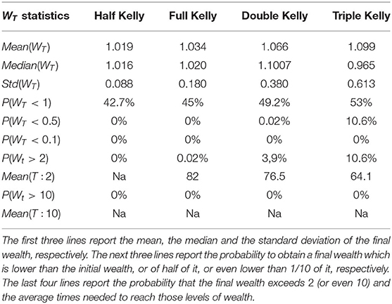
Table 1 shows the value of the final wealth after 100 trades realized on the 10,000 simulated GBM trajectories defined in Equation (14) and obtained from an initial wealth equal to 1.
The results show a trade-off between mean and standard deviation of the final wealth. Increasing the bet size induces an increase in the average final wealth, although the highest median value of the final wealth is obtained from the Full Kelly strategy. Next, the more the amount invested in the stock at each individual trade increases, the more the probability to lose money at the end of 100 trades increases. Moreover, the probability to double the initial wealth increases as the fraction size increases while the time to reach the target level of wealth decreases. Finally, there is no strategy able to increase 10-fold the initial wealth with the number of maximum trades fixed at 100. These results contradict the theory underlying the Kelly criterion and lead us to the conclusion that 100 trades are too few for the criterion to work properly.
3.1.2. 1,000 Trades
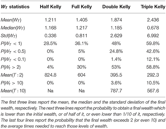
Table 2 shows the results of the final wealth after 1,000 trades realized on the 10,000 simulated GBM trajectories defined in Equation (14) and obtained from an initial wealth equal to 1.
The results, in line with the 100 trades case, still provide evidence about a trade-off between mean and standard deviation and confirm that the Full Kelly strategy has the highest median value of the final wealth compared to the other strategies. Compared to the 100 trades case, both mean and standard deviation increase, whilst the median of the final wealth always increases except in the case of the Triple Kelly. The probability that the final wealth is below the initial one always decreases except in the case of the Triple Kelly. In view of that, it is possible to argue that over betting can still bring high returns in terms of the final wealth but at the cost of a very high risk. Moreover, the probability for the final wealth to exceed a pre-specified target value, particularly Wt > 2, increases in the case of risk-seeking strategies. The riskiest strategies need less time to reach these goals. These results are still not sufficient to support the properties of the Kelly criterion, thus 1,000 days of trades are not enough to be considered as a long term investment in a Kelly's perspective.
3.1.3. From 10,000 to 40,000 Trades
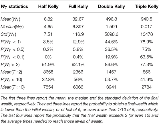
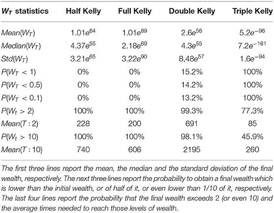
Table 3 reports the information about the final wealth after 10,000 trades realized on the 10,000 simulated GBM trajectories defined in Equation (14) and obtained from an initial wealth equal to 1.
Again, we can notice that mean and standard deviation increase as the bet size increases. This result is consistent with the previous simulations. The full Kelly has the highest median value of the final wealth, whilst the corresponding result for the Triple Kelly is lower than the initial wealth. The probability that the final wealth is below the initial one decreases considerably compared to the previous two simulations except for the Triple Kelly. For the latter, the investor is losing his wealth almost 80% of the times. Thus, over betting three times the optimal Kelly fraction is not really a wise strategy, even for risk seeking investors, because the higher risk is not compensated by a corresponding higher reward. These results demonstrate that 10,000 trades seems sufficient to prove the well-known problem of over betting, but still the Full Kelly does not beat the other strategies.
To overcome this problem we run an additional simulation, but it refers to a very extreme case and cannot be considered as a meaningful and implementable model. Due to consistent reduction in computing power we run the Monte Carlo simulation for 40,000 trades with 1,000 trajectories, and we also used simulated monthly returns, thus simulating a monthly rebalancing between the risky asset and the risk-free asset. This would mean to trade every month for more than 3,000 years. The results of these simulations are shown in Table 4.
In the extreme and unrealistic example represented in Table 4 all the properties of the Kelly criterion are met. The Full Kelly is the one with the highest mean and median value of the final wealth, as well as the fastest one reaching wealth goals besides the Triple Kelly that never reaches the target level and causes initial wealth deterioration 100% of the times. Thus, these results provide evidence that long run had to be really long. In the end, as demonstrated by Breiman [6], the Full Kelly strategy beats all the other essentially different strategies even if we do not know the exact outcomes of the bets but we just know their probability distribution.
In the following, we summarize the main findings of the three experiments based on 100, 1,000, 10,000, and 40,000 trades, respectively.
The results obtained for the short term scenario, i.e., 100 trades, do not support the main property of the Kelly criterion. In this case, the only meaningful outcome is that the Full Kelly has the highest median value of the final wealth, and that over betting leads to higher reward but at the cost of higher risk.
The results do not change much in the 1,000 trades case: over betting still lead to high return but again at the cost of a higher risk, whilst under betting tends to reduce the risk as in the Half Kelly strategy.
In the very long term scenario (40,000 monthly trades) the Full Kelly is finally able to beat any other essentially different strategy. Moreover, the Full Kelly is the fastest strategy to reach any wealth goal, and provides the highest value of the final mean wealth. In contrast, the Triple Kelly strategy implicates sure ruin. The Half Kelly beats the Double Kelly, leading to a higher growth but with a lower risk.
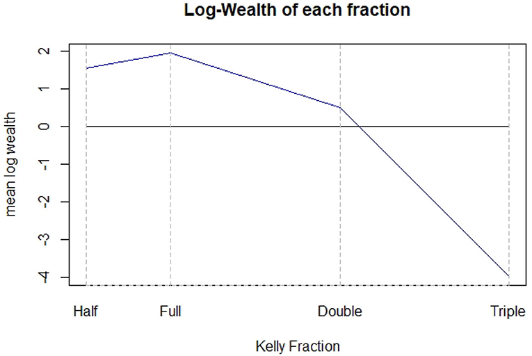
Figure 2 shows the experiment counterpart of Figure 1. For 10,000 trades, i.e., the most plausible scenario for the Kelly criterion to work well, the different values in mean, standard deviation and median obtained from the simulations are summarized in the levels of mean log wealth. The Full Kelly maximizes the expected logarithm of the final wealth, and it is possible to notice that under betting can still have a positive growth. Over betting, instead, requires more attention as it could lead to disastrous events in the long run. This is the case of the Triple Kelly strategy (the final wealth is very close to zero). As for the Double Kelly, the mean final wealth is higher than the initial one but nevertheless lower than that obtained with both the Half and Full Kelly.
3.2. Real Data Examples
In this section, we evaluate the performance of the Kelly Criterion used either on single stocks or on portfolios composed with equities listed in the EuroStoxx50. We evaluate the performance of different portfolios created using the mean-variance approach.
3.2.1. Kelly Criterion When Trading on a Single Equity
We consider Banca Intesa as the reference stock. It concerns one of the major Italian banks and it is listed in both the FTSEMIB and the EuroStoxx50 indexes. Daily returns are computed from the adjusted prices observed on daily basis from January 1, 2007 to December 31, 2018 (2,920 observations). The distribution of the observed returns has mean μ = 0.000407 and variance σ2 = 0.000712. We consider an annual constant risk-free rate of 1%, that converted on daily basis corresponds to: .
To compute the optimal (Full) Kelly fraction we plug the risk/return information into Equation (9)
The trading strategy is implemented as follows. We consider a full Kelly portfolio composed of Banca Intesa and the risk-free asset that is rebalanced in each trading day to keep the portfolio weights of the two assets fixed. The portfolio value at time t + 1 is given by
where rft and rBIt are the observed returns for the risk-free asset and Banca Intesa, respectively, whilst and are their portfolio weights.
This strategy is compared with the Half Kelly, the Triple Kelly and the buy-and-hold strategies considering Banca Intesa as a unique asset. For sake of simplicity, we assume there are no transaction costs, and that the risk-free rate corresponds to the borrowing rate.
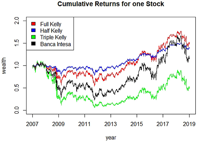
The cumulative returns obtained from the different strategies are represented in Figure 3. The Full Kelly strategy has the highest final wealth, and reaches the maximum wealth during the sample period. The Triple Kelly goes almost close to ruin, thus the investor using this strategy would have lost most of his wealth after 12 years of investment. The Half Kelly has the second highest final wealth and in the periods of high volatility and negative returns is the best-performing strategy. This result supports the motivations underlying the widespread use of this strategy among practitioners. Both Half Kelly and Full Kelly over performed the buy and hold strategy (Banca Intesa), and this finding further supports the good properties of the Kelly criterion.
In Table 5, we report three performance indicators for the compared strategies, namely the Compound Annual Growth Rate (CAGR), the final wealth and the maximum drawdown. The Half and Full Kelly over-perform the Buy and Hold strategy, both w.r.t. CAGR and maximum drawdown. Results obtained for the Triple Kelly portfolio confirm that over-investment can have disastrous outcomes, with a maximum drawdown very close to 95%.

Table 5. Risk-Return performance measurements for the compared strategies in the single equity case (daily data).
Summarizing, this simple example shows that the Kelly Criterion can suggest the optimal way to maximize the final wealth in all cases when the mean and variance of a stock are known or they can be estimated accurately.
In the following, we use real data to compute the optimal Kelly portfolio aimed at maximizing the expected growth rate g* according to Equation (13) and compare these portfolios with that created under the standard Markowitz approach. We perform both an in-sample and out-of-sample analysis either in a static or rolling way.
3.2.2. Kelly vs. Mean-Variance
We compare the portfolio optimized under the Full Kelly criterion and the optimization method introduced in section 2.2.3 with the efficient portfolio optimized using the mean-variance approach on a data set composed of daily returns of 42 equities listed in the EuroStoxx50 index: Adidas, Air Liquide, Allianz, Axa, Banca Intesa, BASF, Bayer, BBVA, BMV, BNP, Carrefour, CRH plc, Deutsche Telekom, Daimler, Danone, Deutsche Bank, Enel, Engie, Eni, EOAN, Generali, Iberdrola, Kering, L'Oreal, LVMH, Munchener Ruck, Nokia, Orange, Philips, Safran, Saint-Gobain, Sanofi, Santander, SAP, Schneider Electric, Siemens Telefonica, Total, Unibail Rodamco Westfield, Unilever, and Vinci. Equities are observed from January 1, 2000 to December 31, 2018. The other equities composing the Eurostoxx50 (Airbus, Anheuser-Busch, Credite Agricole, Endesa, EssilorLuxottica, ING Groep, Societe Generale, and Volskwagen) are excluded from the analysis as they show missing values and/or were included in the index after the year 2000.
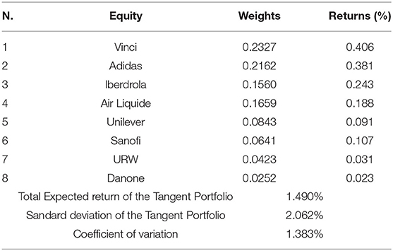
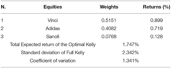
Table 6 shows weights, return and risk of the tangent portfolio (the portfolio that maximizes the Sharpe Ratio) composed considering an annual risk free rate of 1%, whilst Table 7 shows the characteristics of the optimal Kelly portfolio, with no short and no leverage condition.
Results show that the Kelly portfolio is less diversified with respect to the tangent portfolio, as it is composed of three assets only whilst the latter includes eight assets. Comparing the expected returns and risk of the two models, the Kelly portfolio gives the investor a higher expected return of0.256% per month, but it bears a greater standard deviation (2.342%). Nevertheless, the difference in risk is really negligible if considered in relative terms, i.e., comparing the values of coefficient of variation.
These findings are consistent with the previous literature, particularly with Laureti et al. [32] which called this phenomenon “portfolio condensation,” and with Estrada [4] which reports that portfolios built under the Kelly criterion are less diversified, have a higher expected return, and higher risk compared to those composed with the goal of maximizing risk-adjusted returns.
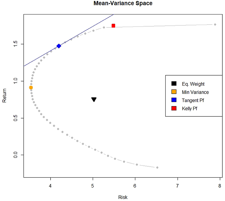
The same findings can be observed in Figure 4. It shows the efficient frontier composed of 50 portfolios optimized using the Markowitz criterion, plus the minimum variance portfolio, the equally weighted portfolio and the tangent portfolio. Moreover, the capital market line and the optimal Full Kelly portfolio are also represented.
From Figure 4, we can see that the optimal Full Kelly portfolio is located on the efficient frontier, but rather far from the capital market line. Its position in the mean-variance space confirms that it shows both a higher risk and a higher return compared to the other represented portfolios.
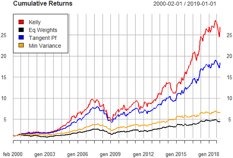
Finally, Figure 5 shows the cumulative returns of the four portfolios previously represented in the mean-variance space (Figure 4).
It is possible to notice that 1 unit of wealth invested in the Full Kelly portfolio grew more than 25 times at the end of the period whilst in the same period the min-variance and the equally-weighted portfolios are valued less than one third of the value of the Kelly portfolio. The latter is also valued more than the tangent portfolio but, consistent with the literature, it presents more pronounced drawdowns.
3.2.3. Rolling Optimization
In the previous section we discuss the similarities and differences of portfolio composed with respect to the Kelly or the Markowitz optimization criteria. In this section, we investigate about the behavior of the two criteria when portfolios are optimized in a dynamic manner using a rolling optimization approach. The latter considers a lookback period th = (t − h,…, t) and defines the portfolio composition at time () according to the following algorithm:
1. Compute mean and variance-covariance matrix of the assets' returns observed in .
2. Compute the portfolio weights using a specific optimization method [Kelly portfolios implemented in Equation (13) or Markowitz] with inputs identified in step 1.
3. Compute portfolio returns in .
4. Repeat steps 1 to 3 for
Basically, at each time point the portfolio is rebalanced based on the results obtained when optimizing w.r.t. data observed in the most recent h time points.
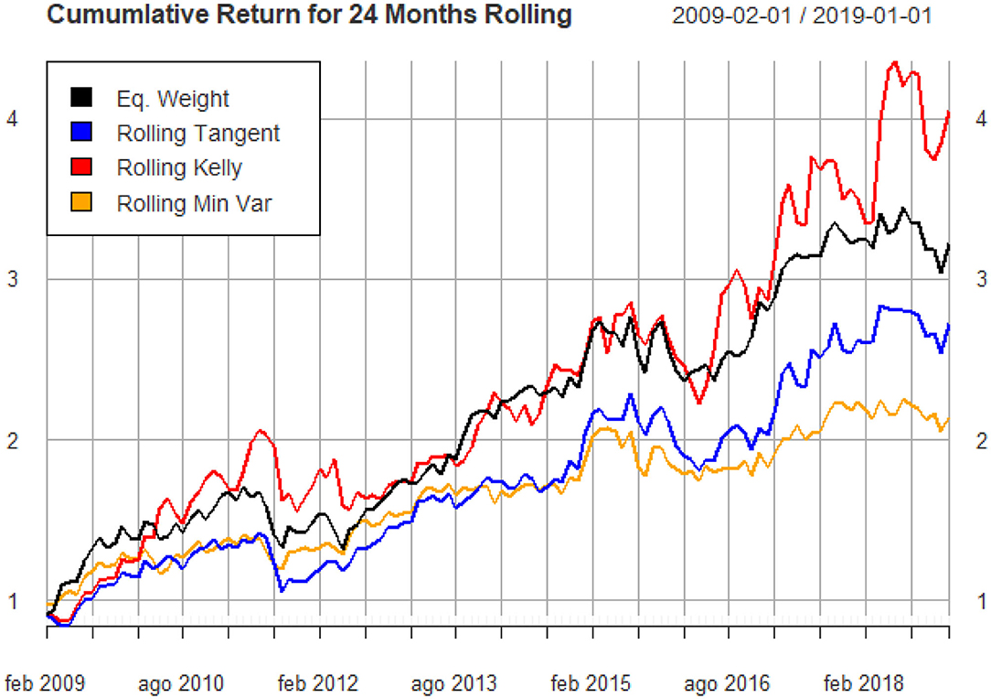
As in the previous section, we use data of the 42 equities listed in the EuroStoxx 50 and consider their monthly returns from January 2007 to December 2018 (144 observations). The rolling lookback period h is set to 24 months (2 years). Thus, we assume the investment starts on the 25-th month and the portfolio is rebalanced monthly. Again, we compare the performances of the tangent portfolio, the minimum variance portfolio and the optimal Full Kelly portfolio. The equally weighted portfolio, rebalanced monthly, is considered the benchmark portfolio.
The results can be seen in Figure 6.
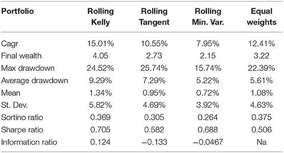
We notice that the only portfolio that beats the benchmark is the optimal Kelly portfolio, and for most of the considered investment horizons it is the one producing the highest cumulative return. The minimum variance and the tangent portfolio follow a very close path, but they are frequently below the equally weighted portfolio. Table 8 shows some statistics of the four portfolios. As expected, the Kelly rolling Portfolio has the highest return and the highest volatility, the maximum drawdown value is similar to that of the tangent portfolio, but it's still higher than the equally weighted and minimum variance one, whilst the average drawdown is highest in the rolling Kelly. This is typical of the Kelly criterion approach. Results also show that the minimum variance portfolio has its typical low-risk characteristic, and in fact it produces the lowest drawdown and both the smallest expected return and volatility. Surprisingly, the tangent portfolio optimized using the Markowitz criterion does not perform well-compared to the others and particularly with respect to the benchmark in terms of expected returns. This result is consistent with the findings of Levy and Duchin [33] who claim that the re-balanced buy and hold portfolio, that they call the “1/N rule” has an important advantage over classical diversification methods: it is not exposed to estimation errors that cause investors who follow for example the Markowitz rules to either over-invest or under-invest in a given security. For this reason, the “1/N rule” may actually outperform the classical diversification methods in the out-of-sample framework.
We also compared the four portfolios in terms of risk measures: we consider the Sortino Ratio, which is used to score a portfolio's risk-adjusted returns with respect to an investment target using downside risk (in our case the risk-free rate is considered as the minimum acceptable return). The equally weighted portfolio is the one with the best performance. This is probably due to the highest diversification. However, all the four considered portfolios have similar values for the Sortino Ratio. If one focuses on the Sharpe Ratio, the portfolios show similar results. The rolling Kelly portfolio is ranked first, whilst the equally weighted is ranked last. The tangent portfolio, although by definition is the one that maximizes the Sharpe Ratio, performs worse compared to the minimum variance and the Kelly portfolio. Table 8 also reports the Information Ratio(IR), which measures the performance of a portfolio compared to a benchmark index, in our case the Equally weighted portfolio, after adjusting for its additional risk. Results for IR shows that the only portfolio having a positive IR, thus over-performing the equally weighted portfolio, is the rolling Kelly whilst the other two portfolios do not consistently beat the benchmark.
3.2.4. Sensitivity Analysis
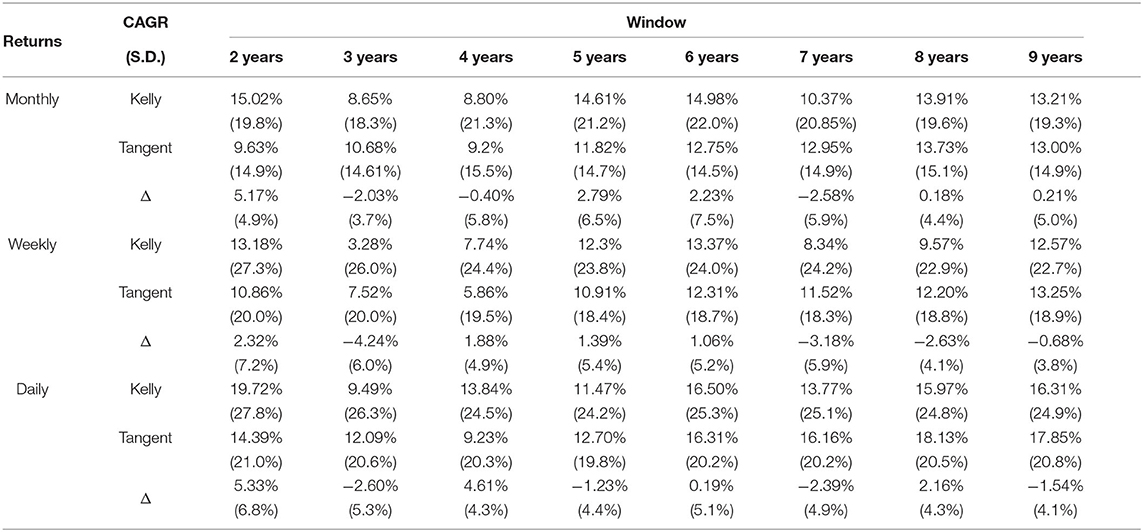
We investigate about the effect of changes in the width of the rolling window or in the frequency of returns on the compound annual growth rate through a sensitivity analysis, whose results are shown in Table 9. We compared the CAGR and the annualized standard deviation of the mean-variance portfolio and of the Kelly portfolio considering different lengths of the window width, ranging from 2 to 9 years. The comparison is made for daily, weekly, and monthly returns, each case inducing daily, weekly, and monthly portfolio rebalancing.
Results in Table 9 reports values of the two metrics (CAGR and annualized standard deviation). It is worth to notice that, using a short window width (2 years of returns) to compute both the expected average returns and variance-covariance matrix, the rolling Kelly portfolio performs outstandingly better than the tangent portfolio. Moreover, the 2-years window width case produces the best performance of the rolling Kelly portfolio despite of both other possible lengths of the window width and the time frequency of returns (daily, weekly, or monthly). The opposite happens for the tangent portfolio: longer windows lead to higher returns. We conjecture that this result is driven by the nature of the Kelly criterion. The latter points out the best size of the bet that, in a series of favorable bets, maximizes the final wealth of the gambler/investor. Thus, it is reasonable to argue that the Kelly criterion is able to capture very well the short term trends of the returns a set of stocks. However, the Kelly portfolio still works fine when the width of the rolling window increases in length, particularly in the case of daily returns. Whereas, CAGR is usually unfavorable if we use weekly returns, thus this choice is somehow discouraged. At the same time, results provide evidence that daily returns lead to portfolios with higher CAGR and higher standard deviation respect to monthly and weekly returns. This is probably from the higher frequency of rebalancing that portfolio optimized on daily returns have compared to those optimized using weekly or monthly returns.
To summarize, the rolling Kelly portfolio performs well if the window width is small (2 years in our study) and it is possible to create small portfolios rebalanced on daily basis. As for the risk side, the rolling Kelly portfolio performs worst compared to the rolling tangent portfolios. In all cases, the standard deviation of Kelly portfolio is larger and of course it tends to grow as the frequency of returns increases.
4. Discussion
This paper shows the theoretical framework of the Kelly criterion as a portfolio optimization method. The criterion was introduced with the purpose of improving information theory, but thanks to the work of various economists and researchers it was applied as a stock market investment strategy. This work also demonstrates, using the Monte Carlo method, all the properties of the Kelly criterion for a continuous probability distribution of returns. We also showed that ignoring the optimal bet size can lead to unpleasant outcomes if the fraction of the capital is greater than that suggested by the Kelly criterion, whilst it can be a reasonable risk adverse strategy if the bet size is lower.
Our simulation and applications on real data show that the use of the Kelly criterion to find the optimal share of wealth to invest in a stock produced results consistent with the literature. The knowledge of the first two moments of the distribution of the returns makes the Kelly criterion able to find the optimal fraction to be invested in a single stock, maximizing the final wealth over a long series of trades. However, bad estimates of mean and variance, or over-betting can lead to unpleasant outcomes, whilst under-betting is a risk controlled strategy. In the multivariate case, we demonstrated that the portfolio constructed under the Kelly criterion lays in the efficient frontier, and it has a higher mean and risk, but is less diversified with respect to the tangent portfolio optimized under the Markowitz model. When used in a dynamic approach, specifically in a rolling window fashion, the portfolio optimized with the Kelly criterion reaches higher CAGR and a poorer drawdown performance respect to the Markowitz portfolios. The same evidence has been provided in Hsieh and Barmish [34]. Increasing the number of trades and the frequency of rebalancing increases the performance of the Kelly portfolio but with higher risk. On the downside, this increasing number of trades increases the transition costs, which were not taken into account in this work. Thus, rebalancing too frequently does not seem a wise decision. From the sensitivity analysis, it appears that rebalancing frequently, i.e., each week, both the Kelly and the Tangent portfolios is not wise. Moreover, the optimization works at its best if the window width is large 2 years and with daily rebalancing.
When we used the Kelly criterion in the real stock market world, our results were coherent with the properties demonstrated in the Monte Carlo simulations, and also coherent with the previous literature. The portfolio optimized with the Kelly criterion, with no short and no leverage constrains, lays on the efficient frontier computed with the Markowitz approach, and is more risky but gives higher reward to the investors respect to the tangent and the minimum variance portfolio. Being placed on the efficient frontier causes the Kelly portfolio to be consistent with the Markowitz mean-variance (M-V) portfolios and thus with the Capital Asset Pricing Model (CAPM) also. Both approaches, MV and CAPM, have been developed within the expected utility theory, but Levy [35] recently demonstrates that MV and CAPM can coexist with Consensus Prospect Theory (CPT). In this respect, it is reasonable to assume that this coexistence is still valid if portfolios are optimized using the Kelly criterion. Overall, the rolling method used to compute the variance-covariance matrix and the mean returns showed that a constrained Kelly optimization is a good method for a dynamic portfolio optimization, but still has pros and cons of the Kelly criterion: high reward and high risk. In our case the Kelly portfolio had higher returns respect to the tangent portfolio constructed under the mean variance approach, but this higher reward comes with a higher volatility and a poor drawdown. Similar results where fund in Kim and Shin [3] and Estrada [4] even if they used a different approach when they compute the optimal Kelly fractions.
If the gamble is favorable or the probability distribution of returns is known, or can it be estimated correctly, no other strategy can beat the Kelly criterion in the long run if it is followed diligently. But this is not a very common case. Estimation errors are not rare and can lead to over betting the optimal fraction, and we have seen that this is not pleasant because it can lead to a lower final wealth or in the worst case to the ruin of the investor. However, optimizing the portfolio with the Kelly criterion is still a valid strategy for risk-seeking investors that also are comfortable with undiversified portfolios, and this strategy can lead to high returns, especially if the market is somehow bullish.
To conclude, we notice that previous literature documents that the Kelly criterion optimization generally provides consolidated results: a high return on the long run, high variance and many losses on the short term. Our future research is addressed to further increase the performance of Kelly portfolios even in the short term. We are currently working on investigating about the benefits on portfolio risk deriving from a robust estimation of the variance-covariance matrix. Moreover, since the Kelly criterion is the best strategy to use on a series of favorable bets, its use in option strategies and derivatives is also under investigation as it could result in maximizing the benefits compared with the traditional trading strategies. Last but not least, we will implement the method introduced in Iorio et al. [36, 37] to select stocks to be included in a Kelly portfolio through P-spline clustering of time series.
Data Availability Statement
The raw data supporting the conclusions of this article will be made available by the authors, without undue reservation.
Author Contributions
AC developed the theoretical formalism, performed the analytic calculations, and performed the numerical simulations. CC supervised the project. All authors contributed to the final version of the manuscript.
Conflict of Interest
The authors declare that the research was conducted in the absence of any commercial or financial relationships that could be construed as a potential conflict of interest.
Acknowledgments
Financial support for this study was provided by a grant from the Department of Business and Economics, University of Cagliari, within the research project Dipartimento di Eccellenza 2018, Grant n. 1.005.14/2019.
References
1. Markowitz H. Portfolio selection. J Finance. (1952) 7:77–91. doi: 10.1111/j.1540-6261.1952.tb01525.x
2. Kelly J Jr. A new interpretation of information rate. Bell Syst Tech J. (1956) 35:917–26. doi: 10.1002/j.1538-7305.1956.tb03809.x
3. Kim G, Shin JH. A comparison of the Kelly criterion and a mean-variance model to portfolio selection with KOSPI 200. Ind Eng Manage Syst. (2017) 16:392–9. doi: 10.7232/iems.2017.16.3.392
4. Estrada J. Geometric mean maximization: an overlooked portfolio approach? J Invest. (2010) 19:134–47. doi: 10.3905/joi.2010.19.4.134
5. Latané HA. Criteria for choice among risky ventures. J Polit Econ. (1959) 67:144–55. doi: 10.1086/258157
6. Breiman L. Optimal gambling systems for favorable games. In: Proceedings of the Fourth Berkeley Symposium on Mathematical Statistics and Probability, Volume 1: Contributions to the Theory of Statistics. Berkeley, CA: University of California Press (1961). p. 65–78.
7. Thorp E. A favorable strategy for twenty-one. Proc Natl Acad Sci USA. (1961) 47:110–2. doi: 10.1073/pnas.47.1.110
8. Thorp EO. The Kelly criterion in blackjack sports betting, and the stock market. In: MacLean LC, Thorp EO, Ziemba WT, editors. The Kelly Capital Growth Investment Crtierion Theory and Practice. Singapore: World Scientific Publishing Co. Pte. Ltd. (2011). p. 789–832. doi: 10.1142/9789814293501_0054
9. Nekrasov V. Kelly Criterion for Multivariate Portfolios: A Model-Free Approach. (2014). Available online at SSRN: http://dx.doi.org/102139/ssrn2259133
10. Fama EF, MacBeth JD. Long-term growth in a short-term market. J Finance. (1974) 29:857–85. doi: 10.1111/j.1540-6261.1974.tb01488.x
11. Maclean LC, Thorp EO, Ziemba WT. Long-term capital growth: the good and bad properties of the Kelly and fractional Kelly capital growth criteria. Quant Finance. (2010) 10:681–7. doi: 10.1080/14697688.2010.506108
12. Ziemba W. Ideas in asset and asset–liability management in the tradition of H.M. Markowitz. In: Guerard JB, editor. The Handbook of Portfolio Construction: Contemporary Applications of Markowitz Techniques. Boston, MA: Springer (2010). p. 213–58. doi: 10.1007/978-0-387-77439-8_9
13. Browne S, Whitt W. Portfolio choice and the Bayesian Kelly criterion. Adv Appl Probabil. (1996) 28:1145–76. doi: 10.1017/S0001867800027592
14. Lo AW, Orr A, Zhang R. The growth of relative wealth and the Kelly criterion. J Bioecon. (2018) 20:49–67. doi: 10.1007/s10818-017-9253-z
15. Ziemba WT. The symmetric downside-risk Sharpe ratio. J Portfolio Manage. (2005) 32:108–22. doi: 10.3905/jpm.2005.599515
16. Thorp EO. Portfolio choice and the Kelly criterion. In: Ziemba WT, Vickson RG, editors. Stochastic Optimization Models in Finance. New York, NY: Academic Press; Elsvier (1975). p. 599–619.
17. Davis M, Lleo S. Fractional kelly strategies for benchmarked asset management. In: The Kelly Capital Growth Investment Criterion Theory and Practice. World Scientific Publishing Co. Pte. Ltd. (2011). p. 385–407. Available online at: https://EconPapers.repec.org/RePEc:wsi:wschap:9789814293501_0027
18. Peterson Z. Kelly's criterion in portfolio optimization: a decoupled problem. J Invest Strat. (2018) 7:53–76. doi: 10.21314/JOIS.2017.097
19. Rising JK, Wyner AJ. Partial Kelly portfolios and shrinkage estimators. In: 2012 IEEE International Symposium on Information Theory Proceedings. Cambridge, MA: IEEE (2012). p. 1618–22. doi: 10.1109/ISIT.2012.6283549
20. Han Y, Yu PLH, Mathew T. Shrinkage estimation of Kelly portfolios. Quant Finance. (2019) 19:277–87. doi: 10.1080/14697688.2018.1483583
21. Hsieh CH, Barmish BR. On drawdown-modulated feedback control in stock trading. IFAC PapersOnLine. (2017) 50:952–8. doi: 10.1016/j.ifacol.2017.08.167
22. Busseti E, Ryu EK, Boyd S. Risk-constrained Kelly gambling. J Invest. (2016) 25:118–34. doi: 10.3905/joi.2016.25.3.118
23. Osorio R. A prospect-theory approach to the Kelly criterion for fat-tail portfolios: the case of Student's t-distribution. Wilmott J. (2009) 1:101–7. doi: 10.1002/wilj.7
24. Aurell E, Baviera R, Hammarlid O, Serva M, Vulpiani A. A general methodology to price and hedge derivatives in incomplete markets. Int J Theor Appl Finance. (2000) 3:1–24. doi: 10.1142/S0219024900000024
25. Wu ME, Chung WH. A novel approach of option portfolio construction using the Kelly criterion. IEEE Access. (2018) 6:53044–52. doi: 10.1109/ACCESS.2018.2869282
26. Wu ME, Hung PJ. A framework of option buy-side strategy with simple index futures trading based on Kelly criterion. In: 2018 5th International Conference on Behavioral, Economic, and Socio-Cultural Computing (BESC). Kaohsiung: IEEE (2018). p. 210–2. doi: 10.1109/BESC.2018.8697308
27. Rotando LM, Thorp EO. The Kelly criterion and the stock market. Am Math Monthly. (1992) 99:922–31. doi: 10.1080/00029890.1992.11995955
28. Black F, Scholes M. The pricing of options and corporate liabilities. J Polit Econ. (1973) 81:637–54. doi: 10.1086/260062
29. R Core Team. R: A Language and Environment for Statistical Computing. Vienna (2019). Available online at: https://www.R-project.org/
30. Berwin A, Turlach R, Weingessel A, Moler C. quadprog: Functions to Solve Quadratic Programming Problems. R package version 1.5-8 (2019). Available online at: https://CRAN.R-project.org/package=quadprog
31. Wuertz D, Setz T, Chalabi Y, Chen W. fPortfolio: Rmetrics–Portfolio Selection and Optimization. R package version 3042.83.1 (2020). Available online at: https://CRAN.R-project.org/package=fPortfolio
32. Laureti P, Medo M, Zhang YC. Analysis of Kelly-optimal portfolios. Quant Finance. (2010) 10:689–97. doi: 10.1080/14697680902991619
33. Levy H, Duchin R. Markowitz's mean-variance rule and the Talmudic diversification recommendation. In: Levy H, Duchin R, editors. The Handbook of Portfolio Construction: Contemporary Applications of Markowitz Techniques. Boston, MA: Springer (2010). p. 97–123. doi: 10.1007/978-0-387-77439-8_4
34. Hsieh CH, Barmish BR. On Kelly betting: some limitations. In: 2015 53rd Annual Allerton Conference on Communication, Control, and Computing (Allerton). Monticello, IL: IEEE (2015). p. 165–72. doi: 10.1109/ALLERTON.2015.7447000
35. Levy H. The Capital Asset Pricing Model in the 21st Century: Analytical, Empirical, and Behavioral Perspectives. Cambdrige, MA: Cambridge University Press (2011).
36. Iorio C, Frasso G, D'Ambrosio A, Siciliano R. A P-spline based clustering approach for portfolio selection. Expert Syst Appl. (2018) 95:88–103. doi: 10.1016/j.eswa.2017.11.031
Keywords: Kelly criterion, portfolio optimization, optimal growth rate, geometric mean-variance, Markowitz, EuroStoxx50
Citation: Carta A and Conversano C (2020) Practical Implementation of the Kelly Criterion: Optimal Growth Rate, Number of Trades, and Rebalancing Frequency for Equity Portfolios. Front. Appl. Math. Stat. 6:577050. doi: 10.3389/fams.2020.577050
Received: 28 June 2020; Accepted: 24 August 2020;
Published: 08 October 2020.
Edited by:
John Guerard, McKinley Capital Management, United StatesReviewed by:
Svetlozar Rachev, Texas Tech University, United StatesAmin Salighehdar, Stevens Institute of Technology, United States
Copyright © 2020 Carta and Conversano. This is an open-access article distributed under the terms of the Creative Commons Attribution License (CC BY). The use, distribution or reproduction in other forums is permitted, provided the original author(s) and the copyright owner(s) are credited and that the original publication in this journal is cited, in accordance with accepted academic practice. No use, distribution or reproduction is permitted which does not comply with these terms.
*Correspondence: Claudio Conversano, Y29udmVyc2FAdW5pY2EuaXQ=
 Andrea Carta
 Claudio Conversano