 Daoping Yu
- School of Computer Science and Mathematics, University of Central Missouri, Warrensburg, MO, United States
In this paper three information criteria are employed to assess the truncated operational risk models. The performances of the three information criteria on distinguishing the models are compared. The competing models are constructed using Champernowne, Frechet, Lognormal, Lomax, Paralogistic, and Weibull distributions, respectively. Simulation studies are conducted before a case study. In the case study, certain distributional models conform to the external fraud type of risk data in retail banking of Chinese banks. However, those models are difficult to distinguish using standard information criteria such as Akaike Information Criterion and Bayesian Information Criterion. We have found no single information criterion is absolutely more effective than others in the simulation studies. But the information complexity based ICOMP criterion says a little bit more if AIC and/or BIC cannot kick the Lognormal model out of the pool of competing models.
1. Introduction
This paper mainly applies model selection information criteria to operational risk models subject to data truncation. In the practice of collecting operational loss data of a bank, certain losses below a threshold value are not recorded. Thus, the data at hand can be viewed as truncated from below. The truncated models, compared to the shifted models and naive models, have been determined to be appropriate to model loss data for operational risk [1].
Model selection differs from model validation. Perhaps there are a few models passing the validation process. Model selection criteria are further used to separate a most suitable model from the rest. Traditional information criteria such as Akaike Information Criterion (AIC) and Bayesian Information Criterion (BIC) have been documented [2] for a banking organization to employ when comparing alternative models. The recent research work of Isaksson [3] and Svensson [4] have explored model selection for operational risk models. Using AIC and/or BIC, they have determined the overall best distributional model(s) for internal data or external data for operational risk in financial institutions.
The purpose of this paper is to assess the effectiveness of information complexity based ICOMP criterion, compared with AIC and/or BIC, to distinguish the fat tailed distributional models for operational risk.
The structure of the remaining of this paper is as follows. In section 2, six candidate distributions for construction of the truncated models of operational risk are reviewed: they are Champernowne distribution, Frechet distribution, Lognormal distribution, Lomax distribution, Paralogistic distribution, and Weibull distribution. In section 3, we give an introduction to such standard information criteria as AIC and BIC for model selection. After reviewing standard information criteria, another information criterion based on information complexity, known as ICOMP, is presented. In section 4, we conduct simulation studies for the six distributional models. In section 5, we walk the readers through the model fitting, model validation, VaR estimation, and model selection procedure, using a real data set for external fraud type of losses in retail banking across commercial banks in China. The practical performance of all information criteria presented in this paper is compared. Concluding remarks are provided in section 6.
2. Parametric Distributions for Operational Risk
The real data of operational losses usually exhibit fat tail properties. The main body of the data are of low severity and high frequency. In other words, operational losses of small sizes occur on a frequent basis. The losses of significantly larger sizes would occur less frequently, but cannot be ignored, since a few extremely large magnitude of losses could be very influential to the financial health and security of a financial institution. A few appropriate distributions for modeling the skewed type of operational loss data have been studied in the literature: for instance, the Champernowne distribution (see for example, [5]), the Lognormal distribution (see for example, [6]), and the Lomax distribution (also known as two-parameter Pareto distribution) as a special case of the Generalized Pareto Distribution (see for example, [7]), etc. There are a few other distributions that are suitable to model fat tailed risks, such as the Frechet distribution, the Paralogistic distribution, and the Weibull distribution (see for instance, [8]).
2.1. Champernowne Distribution
The Champernowne distribution is originally proposed in the study of income distribution, and it is a generalization of the logistic distribution, firstly introduced by an econometrician D. G. Champernowne [9, 10], in the development of distributions to describe the logarithm of income. The Champernowne distribution has probability density function (pdf)
and cumulative distribution function (cdf)
where α > 0 is the shape parameter and M > 0 is another parameter that represents the median of the distribution. The Champernowne distribution looks more like a Lognormal distribution near x value of 0 when α > 1, while converging to a Lomax distribution in the tail. In addition, by inverting the cdf given in (2) one obtains the quantile function (qf) as
For more details about the application of Champernowne distribution to operational risk modeling, readers are referred to a monograph (see [5]).
2.2. Frechet Distribution
The Frechet distribution is also known as the inverse Weibull distribution. The pdf of the two-parameter Frechet distribution is given by
and the cdf is given by
The qf is found by inverting (5) and given by
For the Frechet distribution, α > 0 is the shape parameter, and θ > 0 is the scale parameter.
2.3. Lognormal Distribution
The Lognormal distribution with parameters μ and σ is defined as the distribution of a random variable X whose logarithm is normally distributed with mean μ and variance σ2. The two-parameter Lognormal distribution has pdf
where −∞ < μ < ∞ is the location parameter and σ > 0 is the scale parameter.
The two-parameter Lognormal distribution has cdf
and by inverting (8), the quantile function
is obtained. Here Φ and Φ−1 denote the cdf and qf of the standard normal distribution, respectively.
2.4. Lomax Distribution
The pdf of the two-parameter Pareto distribution, also called Lomax distribution, is given by
and the cdf is given by
and the qf is found by inverting (11) and given by
We refer readers to Arnold [11] for more details of Pareto distributions, and see Klugman et al. [8] for the applications of Pareto distributions to insurance loss modeling.
2.5. Paralogistic Distribution
The pdf of the two-parameter Paralogistic distribution is given by
and the cdf is given by
and the qf is found by inverting (14) and given by
The Paralogistic distribution is characterized by the shape parameter α > 0 and the scale parameter θ > 0.
2.6. Weibull Distribution
The pdf of the two-parameter Weibull distribution is given by
and the cdf is given by
and the qf is found by inverting (17) and given by
The parameter α > 0 characterizes the shape of the Weibull distribution, and the parameter θ > 0 characterizes the scale.
3. Information Criteria
Given a data set, X1, …, Xn, the amount of objective information contained in the data is fixed. However, different models may be fitted to the same data set in order to extract the information. We want to select the model that best approximates the distribution of the data. There are various information criteria for model selection, such as the Akaike Information Criterion [12], Bayesian Information Criterion [13], and Information Complexity (ICOMP) [14, 15]. The defining formulas of all these three contain negative double log-likelihood.
Let be the likelihood function of a model with k parameters based on a sample of size n, and let , …, denote the corresponding estimators of those parameters using the method of Maximum Likelihood Estimation (MLE).
The AIC is defined as:
The BIC is defined as:
The ICOMP is defined as:
where
with s, tr, and det denoting the rank, trace, and determinant of I−1 (the inverse of Fisher information matrix), respectively.
Using those information criteria, the preferred model is the one that minimizes AIC, BIC, or ICOMP. In general, it is known that when the number of parameters increases, the model likelihood increases as well. We see that there is a competition between the increase in the log-likelihood value and the increase in the number of model parameters in the AIC and BIC formulas. If the increase in the log-likelihood value is not sufficient to compensate the increase in the number of parameters, then it is not worthwhile to have the additional parameters. Note also that the BIC criterion penalizes the model dimensionality more than AIC for logn > 2.
ICOMP penalizes the interdependencies among parameter estimators of MLE, i.e., the complexity of variance-covariance structure of model's maximum likelihood estimators via the inverse Fisher information matrix. It is a generalization of the maximal information measure proposed by van Emden [16]. Let In = n·I denote the Fisher information matrix based on a sample of size n. The ICOMP penalty term is a function of the matrix I rank, trace and determinant. The minimum value of the penalty term is zero, which is reached when the variances of parameter estimators are equal and the covariances are zeros. The ICOMP criterion is very effective for regression-type models.
4. Simulation Studies
To get an idea of how each of AIC, BIC, and ICOMP performs in selecting distributional models, let us first of all conduct some simulation studies. The purpose of the simulation is to see which criterion can capture the true underlying distribution from which the data is generated from.
We are going to simulate data from each of Champernowne, Frechet, Lognormal, Lomax, Paralogistic, and Weibull distributions, with specified parameter values. For each distribution, the simulation is done twice, the first time with a relatively small sample size of 100, and the second time with a relatively large sample size of 1,000. Thus, there are in total 12 data sets being simulated. Then we fit all six distributions to each of the 12 simulated data sets.
In Tables 1–12, we will present the results of the simulation studies, about the performance of all three information criteria.
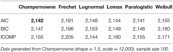
Table 1. Simulation: Information criteria for Champernowne, Frechet, Lognormal, Lomax, Paralogistic, and Weibull models.
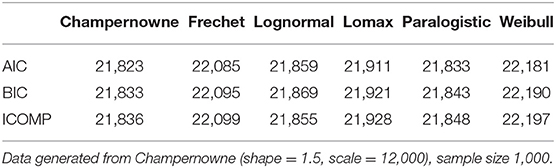
Table 2. Simulation: Information criteria for Champernowne, Frechet, Lognormal, Lomax, Paralogistic, and Weibull models.
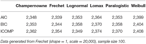
Table 3. Simulation: Information criteria for Champernowne, Frechet, Lognormal, Lomax, Paralogistic, and Weibull models.
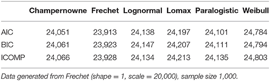
Table 4. Simulation: Information criteria for Champernowne, Frechet, Lognormal, Lomax, Paralogistic, and Weibull models.
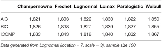
Table 5. Simulation: Information criteria for Champernowne, Frechet, Lognormal, Lomax, Paralogistic, and Weibull models.

Table 6. Simulation: Information criteria for Champernowne, Frechet, Lognormal, Lomax, Paralogistic, and Weibull models.

Table 7. Simulation: Information criteria for Champernowne, Frechet, Lognormal, Lomax, Paralogistic, and Weibull models.
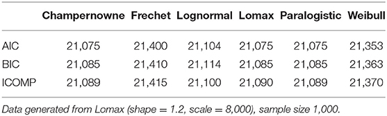
Table 8. Simulation: Information criteria for Champernowne, Frechet, Lognormal, Lomax, Paralogistic, and Weibull models.
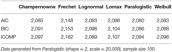
Table 9. Simulation: Information criteria for Champernowne, Frechet, Lognormal, Lomax, Paralogistic, and Weibull models.
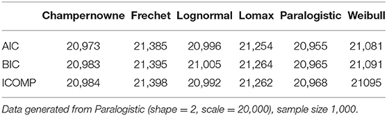
Table 10. Simulation: Information criteria for Champernowne, Frechet, Lognormal, Lomax, Paralogistic, and Weibull models.
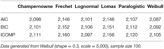
Table 11. Simulation: Information criteria for Champernowne, Frechet, Lognormal, Lomax, Paralogistic, and Weibull models.
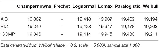
Table 12. Simulation: Information criteria for Champernowne, Frechet, Lognormal, Lomax, Paralogistic, and Weibull models.
In Table 1, AIC values of 2,142 and 2,141 are both regarded as the smallest AIC values since the difference in a magnitude of one is too small and that might be due to round up of decimals. That tiny difference is insignificant. The same logic applies to the lowest BIC values of 2,147 and 2,146. When the sample size is 100, AIC and BIC cannot separate the true Champernowne model from the Paralogistic model. ICOMP tends to favor the Lognormal more than all other models, even though the true model is Champernowne instead of Lognormal. This bias can be corrected by increasing the sample size.
In Table 2, across each row of the three information criteria, the lowest value has been highlighted. All the three information criteria are able to distinguish the true Champernowne model from the other models, if the data is generated with a large sample size of 1,000.
From Table 3, AIC and BIC can determine the best model that is consistent with the underlying true model that generates the data, since the true Frechet model produces the lowest AIC and BIC values among all models. ICOMP says the Lognormal model has the smallest information complexity value, while the true Frechet model turns out to have the second lowest complexity value. This error may be due to the relatively small sample size of 100, and it can be eliminated by increasing the sample size to 1,000, which can be seen in the following table.
When the sample size is 1,000, all AIC, BIC, and ICOMP criteria are successful in identifying the Frechet model as the true model from which the data is generated. This is supported by the lowest values of all information criteria for the Frechet model in Table 4.
In Table 5, we have highlighted a few lowest values of AIC and/or BIC, ignoring the slight difference of one in the values, perhaps due to round up error. It seems that neither AIC nor BIC can separate the true Lognormal model from the other two competing models: the Champernowne model and the Paralogistic model, because all three models produce the lowest AIC and BIC values. ICOMP successfully distinguishes the true Lognormal model from all other models. This simulation study of fitting various models to Lognormal data of sample size 100 suggests that ICOMP is indeed more effective than AIC and BIC to identify the true Lognormal model when the sample size is as small as 100. But this advantage of ICOMP may disappear if we increase the sample size to 1,000, as shown in the next table.
The Lognormal model produces the lowest AIC value, the lowest BIC value, and the lowest ICOMP value, as indicated in Table 6. Thus, all three information criteria successfully select the true underlying model that generates the data, when the true model is Lognormal and the sample size is 1,000.
From Table 7, we can tell that AIC and BIC fail to distinguish among the Champernowne model, the true Lomax model, and the Paralogistic model. We ignore the difference of one in the values that may be due to round up error, and those highlighted values are treated as the smallest ones in that particular row. ICOMP has a biased favor toward the Lognormal model, suggested by the lowest ICOMP value of 2,047 produced by the Lognormal model. However, the true model is Lomax instead of Lognormal. This type of error will go away if the sample size is bigger as indicated in the coming table.
When the true model that generates the data is Lomax, even if the sample size is as large as 1,000, none of AIC, BIC, or ICOMP seems to be able to distinguish the competing three different models: they are the Champernowne model, the true Lomax model, and the Paralogistic model, since they all produce the lowest information criteria values across each row in Table 8. The magnitude of one in the difference of the highlighted values may be subject to round up issues, and such tiny differences do not say much about distinguishing the models.
When the sample size is 100, AIC and BIC can weakly identify the true Paralogistic model that generates the data, since the Paralogistic model produces the smallest AIC and BIC values in Table 9. The reason we say weakly identifying the true model is because the AIC and BIC values of a competing Weibull model are close to those of the true model. However, ICOMP makes a wrong decision to select the Lognormal model (with the lowest ICOMP value of 2,089), even though the ICOMP value (2,094) of the true Paralogistic model comes as the next lowest. ICOMP will make a right decision when the sample size is increased to 1,000 as in the subsequent table.
When the sample size is as large as 1,000, all AIC, BIC, and ICOMP can correctly identify that the true underlying process that generates the data is the Paralogistic model, which has the lowest information criteria values as highlighted in Table 10.
From Table 11, you can tell that AIC and BIC are able to identify the true Weibull model that has generated the data of a relatively small sample size 100, since the Weibull model produces the lowest AIC and BIC values. But ICOMP fails to do so, and ICOMP erroneously picks the Lognormal model (with the lowest ICOMP value of 2,097) and puts the true Weibull model (with the next lowest ICOMP value of 2,105) in the second place.
Fortunately, when the sample size increases from 100 to 1000, ICOMP seems to correct its mistake as of wrongly picking the Lognormal model in the previous table, and now ICOMP also identifies the true Weibull model that has generated the data. AIC and BIC are still working well. All three information criteria end up to have the smallest value for the Weibull model. By the way, in this Table 12, there are no values produced for the Frechet model, since the numerical procedure in maximizing the log-likelihood does not converge. Obviously, when the sample size is 1,000, the Frechet model is definitely not a good fit for the data generated from the Weibull model.
Even if we have only presented 12 tables as above, more simulation studies can be done across a wide range of the parameter values for each distribution, and ICOMP still exhibits a tendency to favor the Lognormal model when the sample size is small. That sort of tendency can disappear when the sample size gets large enough.
Let us make a remark here. When the true data generating process is a Lognormal model, ICOMP beats AIC and BIC if the sample size is small. When the data of small sample size is simulated from another distribution, ICOMP might lose the competition to AIC and/or BIC.
5. Case Study: External Fraud Risk
In this section, we illustrate the model performance on the real data. We walk through the entire process of modeling, beginning with model fitting and model validation, then Value-at-Risk (VaR) estimation, and ends up with model selection using various information criteria.
We have collected data for operational losses of external fraud type in retail banking in branches of major commercial banks of China in 2009–2015. We have recorded the amount of principal indemnification involved in each event. If a savings account holder or a debit card holder loses their money of deposit due to external fraud, a certain proportion of the original loss amount of principal deposit may be indemnified or reimbursed by the bank to mitigate the loss of bank customers. That proportion is determined by the court in accord with how much responsibility the bank is supposed to assume during the events of external fraud. Usual proportion numbers could be 100, 90, 80, 70, 50, or 0%. There are 181 data points that represent the cost of debit card or savings account external fraud events for branches of major commercial banks in China. The cost measure is in Chinese Yuan (RMB) currency. Even though the data have been collected over a span of a few years, the loss sizes are not scaled for inflation. Also the legal costs, involved in the law sue process, are not included. To illustrate the impact of data modeling threshold on the considered models, we split the data set into two portions: losses that are at least 26,000 RMB, which will be regarded as observed and used for model building and VaR estimation; and losses that are below 26,000 RMB, which will be treated as unrecorded by the bank or unobserved. The modeling threshold is a different concept from the reporting threshold: the former is the threshold chosen by the model builders, and the latter is the threshold chosen by each individual bank. We use a modeling threshold of 26,000 RMB just for demonstration purposes. Such a choice of modeling threshold results in 103 observed losses. A quick summary statistics of the 103 observed data shows that it is right-skewed and tentatively heavy-tailed, with the first quartile 40,085, median 72,000, and the third quartile 220,879; its mean is 342,838, standard deviation 944,314, and skewness 5.731.
Such a real dataset is used to conduct the case study, and we consider three distributional models; they are Champernowne, Lomax, and Lognormal models. MLE estimators are solved numerically, when explicit formulas can not be obtained for maximization of the log-likelihood functions. In Table 13, we report the resulting MLE parameter estimates. Further, we assess all models using the visual inspection in Figures 1–6 and formal goodness-of-fit test statistics. The KS and AD goodness-of-fit test statistics are given in Table 14. The VaR estimates are provided in Table 15. Finally the information criteria values are summarized in Table 16.
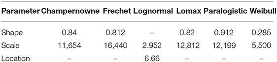
Table 13. Parameter MLEs using truncated approach of the Champernowne, Frechet, Lognormal, Lomax, Paralogistic, and Weibull models.
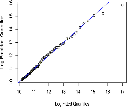
Figure 1. Champernowne QQ-plot.

Figure 2. Frechet QQ-plot.

Figure 3. Lognormal QQ-plot.

Figure 4. Lomax QQ-plot.
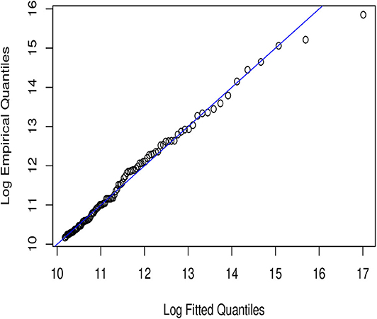
Figure 5. Paralogistic QQ-plot.
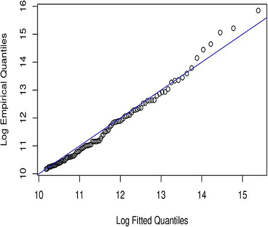
Figure 6. Weibull QQ-plot.

Table 14. The KS and AD statistics for the fitted models, using truncated approach.
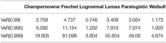
Table 15. External Fraud Risk: VaR(β) estimates, measured in millions and based on the fitted models, using truncated approach.
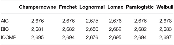
Table 16. External Fraud Risk: Information criteria for truncated Champernowne, Frechet, Lognormal, Lomax, Paralogistic, and Weibull models.
5.1. Model Fitting
Using the 103 observations of the aforementioned construction of dataset, exceeding (inclusively) the modeling threshold 26, 000 Chinese RMB, we fit the Champernowne, Frechet, Lognormal, Lomax, Paralogistic, and Weibull distributions to the data by the truncated approach. The values of parameter estimators are obtained using numerical procedure, when there are no closed form formulas for the parameter estimators. The results are reported in the following table.
For the truncated Champernowne model, the shape parameter estimate is 0.84, and the scale parameter estimate 11,654 is an estimate of the median of the fitted Champernowne distribution. For the truncated Frechet model, the shape parameter estimate is 0.812, and the scale parameter estimate is 16,440. For the truncated Lognormal model, the location parameter estimate of the Lognormal distribution is 6.66, and the scale parameter estimate is 2.952. For the truncated Lomax model, the shape parameter estimate is 0.82, and the scale parameter estimate is 12,812, which in general is not the median estimate unless the shape parameter were exactly equal to one. The shape parameter estimate of the Champernowne model 0.84 seems pretty close to the shape parameter estimate 0.82 of the Lomax model. If we compare the cdf of the Champernowne distribution with that of the Lomax distribution, we could find that they would coincide when the shape parameter α of both were equal to one. For the truncated Paralogistic model, the shape parameter estimate is 0.912, and the scale parameter estimate is 12,199. For the truncated Weibull model, the shape parameter estimate is 0.285, and the scale parameter estimate is 5,500.
5.2. Model Validation
To validate the fitted models we employ visual inspection tools like quantile-quantile plots (QQ-plots) and furthermore two goodness-of-fit test statistics, Kolmogorov-Smirnov (KS) test statistic and Anderson-Darling (AD) test statistic.
In Figures 1–6, we present plots of the fitted-versus-empirical quantiles for the six truncated distributional models. In all the plots both fitted and empirical quantiles have been taken the logarithmic transformation. It seems hard to distinguish the truncated Champernowne (Figure 1), Frechet (Figure 2), Lomax (Figure 4), and Paralogistic (Figure 5) models, as indicated by the graphical inspection of QQ-plots. The truncated Lognormal (Figure 3) model looks good overall by examining the QQ plot visually. The truncated Weibull (Figure 6) model has the QQ plot a little bit further away from the identity line compared to the other five models.
Looking at Figure 1, all points except for the two most extremely large observations lie nearly on or very close to the identity line. Compared with Figure 1 fitting the truncated Champernowne model, we see that Figure 3 indicates a slightly better fit of the truncated Lognormal model in the most extreme right tail (for the largest two observations) because those two points in Figure 3 get closer to the identity line compared to in Figure 1. However, such improvement comes at the cost of a slightly worse fit of the next few observations just below the largest two.
Visual inspection of Figures 1, 4 tells us that they look very similar to each other. This is consistent with what we have observed in the closeness of parameter estimates in Table 13 between the truncated Champernowne model and the truncated Lomax model.
The KS goodness-of-fit test statistic measures the maximum absolute distance between the fitted cdf and the empirical cdf. The AD goodness-of-fit test statistic measures the cumulative weighted quadratic distance (placing more weight on tails) between the fitted cdf and the empirical cdf. The KS and AD statistics have been evaluated using the MLE parameter estimates from Table 13. The following is the table of the KS statistics and the AD statistics for each of the fitted models.
From Table 14, it looks like that all fitted models have low KS and AD values except that the Weibull model produces relatively higher values of KS and AD statistics than the other models. This is consistent with the visual inspection of the QQ-plots.
5.3. VaR Estimates
The final product of operational risk modeling is VaR estimation, built upon the parameter estimates of the fitted models. The concept of VaR is useful in both finance and insurance, and let's define VaR as follows: Let 0 < β < 1. VaR is defined as
where F−1(β) denotes a quantile evaluated at level β of the cumulative distribution function F, and F−1 is a notation used for the generalized inverse of F.
Having gone through the model fitting and model validation, we now are ready to compute the estimates of VaR(β) for all three models. We summarize the results in Table 15.
From Table 15 we see that the considered six models, five of which exhibited nearly as good fit as one another to the studied data, produce substantially different VaR estimates, especially at the very extreme right tail. For example, the Frechet model produces the most conservative VaR estimates at all three levels. The Frechet distribution comes from the family of distributions to model extreme values. The fitted Frechet model turns out to be more heavy-tailed than the other fitted models. On the other hand, the fitted Lognormal model ends up to be less heavy-tailed than the others, and Lognormal VaR values are smaller than the VaR values of other models. For instance, the 99.9% VaR of the truncated Lognormal model is 3.8 million RMB; while it is 18.9 million RMB for the truncated Champernowne model and 55.8 million RMB for the truncated Lomax model. The 99% VaR and 99.5% VaR of the six models maintain the same order of ranking, but the magnitude of gap is not as much as in the highest level of 99.9% VaR. Despite producing very different VaR estimates, we will see in the following section that the six models are very close in terms of the values of information criteria, with an exception for ICOMP of the Lognormal model.
5.4. Information Criteria Results
Finally, in Table 16 we present the values of all information criteria considered in this paper for the truncated Champernowne, Frechet, Lognormal, Lomax, Paralogistic, and Weibull models. The log-likelihood function has been obtained using the truncated distributional approach. Likewise, the Fisher information matrix I(θ1, …, θk) has been derived using the truncated likelihood for the respective parametric distributions.
As we can see from Table 16, the six models are indistinguishable using traditional information criteria such as AIC and BIC, since the values of each criterion are very close for all models. In particular, a slight difference in the AIC values with a magnitude of 1 out of more than 2,000 provides little evidence. It is very similar if we look at the difference of 1 or 2 in the BIC values. The use of the more refined information measure ICOMP does not help among the truncated Champernowne, Frechet, Lomax, Paralogistic, and Weibull models, but has the ability to distinguish the truncated Lognormal model from the other five models. The ICOMP favors the truncated Lognormal model since it produces significantly lower value of ICOMP than the other five models. We can see there is a difference of no <18 out of roughly twenty six hundred, which contrasts that tiny difference in the values of AIC and/or BIC.
6. Concluding Remarks
In this paper, we have studied the problem of model selection in operational risk modeling, which arises due to that various truncated models are all validated but cannot be distinguished. Through the numerical illustrations of simulation studies and a case study in the previous two sections, the performances of the traditional well-known model selection criteria such as Akaike Information Criterion (AIC) and Bayesian Information Criterion (BIC) and another information criterion based on Information Complexity (ICOMP) have been assessed and compared.
We summarize our conclusions as follows. Is ICOMP really credible when choosing a Lognormal model? It depends on the size of the sample, and also relies on whether or not the Lognormal model gets kicked out of the pool of candidate models by AIC and/or BIC. Simulation studies have shown that when the true underlying model is Lognormal and the sample size is 100, ICOMP can successfully identify the Lognormal as the true model, while AIC and/or BIC cannot distinguish the Lognormal model from some of the other models (for example, the Champernowne model, and the Paralogistic model). However, when the sample size in the simulation increases to 1,000, AIC and/or BIC can also successfully separate the true Lognormal model from other models. In this way, when the sample size is 1,000, ICOMP loses its competitive advantage. On the other hand, when the underlying true model is Champernowne, Frechet, Lomax, Paralogistic, or Webull, instead of Lognormal, if the sample size is set to be 100, ICOMP will still erroneously choose Lognormal as the winning model, while AIC and/or BIC will not make such a mistake. Fortunately, this disadvantage of ICOMP will disappear when the sample size increases to 1,000. The reason why ICOMP prefers the Lognormal model so much is probably because the information complexity of the Lognormal variance covariance matrix is simpler than other models.
In order to make full use of the advantages of all the three information criteria and avoid the disadvantages of them, a large sample size is desirable. Otherwise, caution has to be used when the sample size of data at hand is small, for which we propose two stages of model selection. In the first stage, we use AIC and/or BIC to select the best model. If it turns out that AIC and/or BIC are successful, then we use ICOMP to strengthen the selection of the best model. Otherwise, if AIC and/or BIC fails, we will enter the second stage. Due to the failure of AIC and/or BIC, there must be several indistinguishable competing models. We consider two different situations. One situation is that AIC and/or BIC have kicked the Lognormal model out from the candidate pool, if so then we cannot continue to use ICOMP to avoid ICOMP choosing the Lognormal by mistake. The other situation is that after using AIC and/or BIC, the Lognormal is still surviving in the pool of candidate models, then ICOMP may be used further.
Data Availability Statement
The original contributions presented in the study are included in the article/supplementary material, further inquiries can be directed to the corresponding author/s.
Author Contributions
The author confirms being the sole contributor of this work and has approved it for publication.
Conflict of Interest
The author declares that the research was conducted in the absence of any commercial or financial relationships that could be construed as a potential conflict of interest.
Acknowledgments
The author thanks the referees for their review and comments which have helped the author significantly improve the paper.
References
1. Yu D, Brazauskas V. Model uncertainty in operational risk modeling due to data truncation: a single risk case. Risks. (2017) 5:49. doi: 10.3390/risks5030049
2. Basel Coordination Committee. Supervisory guidance for data, modeling, and model risk management under the operational risk advanced measurement approaches. Basel Coord Committ Bull. (2014) 14:1–17. Available online at: https://www.federalreserve.gov/bankinforeg/basel/files/bcc1401.pdf.
3. Isaksson D. Modelling IT risk in banking industry: A study on how to calculate the aggregate loss distribution of IT risk (Thesis). Jönköping University, Jönköping, Sweden (2017).
4. Svensson KP. A Bayesian approach to modeling operational risk when data is scarce (Thesis). Lund University, Lund, Sweden (2015).
5. Bolance C, Guillen M, Gustafsson J, Nielsen JP. Quantitative Operational Risk Models. Boca Raton, FL: CRC Press (2012).
6. Cavallo A, Rosenthal B, Wang X, Yan J. Treatment of the data collection threshold in operational risk: a case study with the Lognormal distribution. J Oper Risk. (2012) 7:3–38. doi: 10.21314/JOP.2012.101
7. Horbenko N, Ruckdeschel P, Bae T. Robust estimation of operational risk. J Oper Risk. (2011) 6:3–30.
8. Klugman SA, Panjer HH, Willmot GE. Loss Models: From Data to Decisions. 4th Edn. Hoboken, NJ: Wiley (2012).
12. Akaike H. Information theory and an extension of the maximum likelihood principle. In: Second International Symposium on Information Theory. Petrox BN, Csaki F, Editors. Budapest: Academiai Kiado (1973). p. 267–81.
14. Bozdogan H. ICOMP: A new model selection criteria. In: Bock H, Editor. Classification and Related Methods of Data Analysis. Amsterdam: Elsevier Science Publishers B.V. (1988) 599–608.
15. Bozdogan H. On the information-based measure of covariance complexity and its application to the evaluation of multivariate linear models. Commun Stat Theor Methods. (1990) 19:221–78.
Keywords: information criteria, model selection, operational risk, truncated models, Value at Risk (VaR)
Citation: Yu D (2020) Comparing Model Selection Criteria to Distinguish Truncated Operational Risk Models. Front. Appl. Math. Stat. 6:28. doi: 10.3389/fams.2020.00028
Received: 01 May 2020; Accepted: 01 July 2020;
Published: 04 August 2020.
Edited by:
Lawrence Kwan Ho Ma, Hong Kong Blockchain Society, Hong KongReviewed by:
Dimitrios D. Thomakos, University of Peloponnese, GreeceSimon Grima, University of Malta, Malta
Copyright © 2020 Yu. This is an open-access article distributed under the terms of the Creative Commons Attribution License (CC BY). The use, distribution or reproduction in other forums is permitted, provided the original author(s) and the copyright owner(s) are credited and that the original publication in this journal is cited, in accordance with accepted academic practice. No use, distribution or reproduction is permitted which does not comply with these terms.
*Correspondence: Daoping Yu, ZHl1QHVjbW8uZWR1