Deep Net Tree Structure for Balance of Capacity and Approximation Ability

Deep learning has been successfully used in various applications including image classification, natural language processing and game theory. The heart of deep learning is to adopt deep neural networks (deep nets for short) with certain structures to build up the estimator. Depth and structure of deep nets are two crucial factors in promoting the development of deep learning. In this paper, we propose a novel tree structure to equip deep nets to compensate the capacity drawback of deep fully connected neural networks (DFCN) and enhance the approximation ability of deep convolutional neural networks (DCNN). Based on an empirical risk minimization algorithm, we derive fast learning rates for deep nets.

1. Introduction

Deep learning [1], a learning strategy based on deep neural networks (deep nets), has recently made significant breakthrough on bottlenecks of classical learning schemes, such as support vector machines, random forests and boosting algorithms, by demonstrating its remarkable success in such research areas as computer vision [2], speech recognition [3], and game theory [4]. Understanding the theory of deep learning has recently triggered enormous research activities in communities of statistics, optimization, approximation theory, and learning theory. Continually rapid developments on the deep learning methodology as well as its rationality verifications gradually uncover its mysterious veils.

Depth and structure of deep nets are two crucial factors in promoting the development of deep learning [5]. The necessity of depth has been rigorously verified from the viewpoints of approximation theory and representation theory, via showing the advantages of deep nets in localized approximation [6], sparse approximation in the frequency domain [7, 8], sparse approximation in the spatial domain [9], manifold learning [10, 11], hierarchical structures grasping [12, 13], piecewise smoothness realization [14], universality with bounded number of parameters [15, 16] and rotation invariance protection [17]. We refer the readers to Pinkus [18] and Poggio et al. [19] for details on the theoretical advantages of deep nets over shallow neural networks (shallow nets). The gain in approximation and feature extraction inevitable leads to large capacity of deep nets, making the derived estimators sensitive to noise accumulated from significant increase amount of computation. In particular, under some capacity measurements like the number of linear regions [20], Betti numbers [21], and number of monomials [22], it is well-known that while the capacity of deep nets increases exponentially with respect to depth and polynomially with respect to width, the increase in depth of the network brings additional risk in stability, additional difficulty in designing learning algorithms, and may result in large variance. In this regard, we would like to point out that although there are the same number of free parameters in neural networks presented in Figure 1, the capacity of the network in Figure 1A is much larger than that in Figure 1B.

FIGURE 1

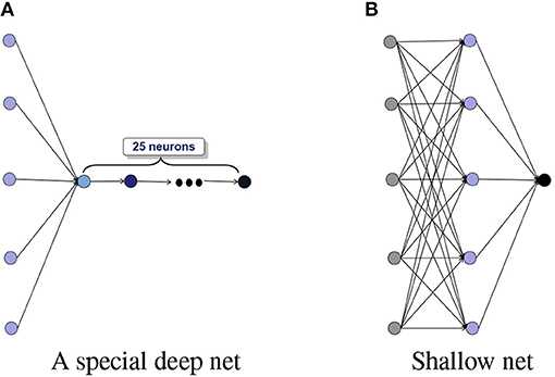
Figure 1. Deep nets vs. shallow nets. (A) A special deep net. (B) Shallow net.

Fortunately, the structure, reflected by the layer-to-layer conjunction rule, compensates for the capacity drawback of deep nets and allows deep learning feasible and even practical. Two dominant structures of deep nets, as shown in Figure 2, are the deep fully connected neural networks (DFCN) and deep convolutional neural networks (DCNN). While the pros of DFCN is its excellent approximation ability, since all the conjunctions are considered in this structure, its cons, however, lies in the extremely large capacity, leading to scalable difficulty and large variance from the learning theory viewpoint [23]. On the other hand, the advantage of DCNN is its small number of free parameters as a result of sparse connectivity and weight-sharing mechanisms. For example, there are 2 free parameters in each layers for a DCNN with filter length 2 (see Figure 2B). Such a parameter reduction certainly brings the benefit in stability and consequently small variance. However, it is questionable if DCNN could maintain the attractive approximation ability of DFCN. Indeed, with the exception of the universal approximation property and approximation rate estimates [24, 25], there is insufficient theoretical study in the assessment of the approximation capability of DCNN. Thus, equipping deep nets with an appropriate structure to reduce the number of parameters of DFCN while enhancing the approximation ability of DCNN requires some desirable balance of the bias and variance in the learning process.

FIGURE 2

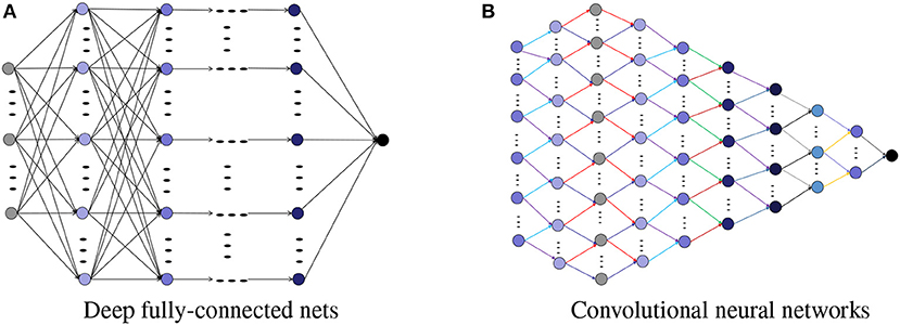
Figure 2. Structures for deep nets. (A) Deep fully-connected nets. (B) Convolutional neural networks.

In this paper, we propose an appropriate structure to equip deep nets with a combination of some smaller variance provided by DCNN and a corresponding less bias advantage of DFCN. Two important ingredients of our approach are feature grouping via dimensionality-leveraging and tree-type feature extraction. Our construction is motivated by the structures of deep nets presented in Chui et al. [6] and Lin [9] for the realization of locality and sparsity features. As shown in Figure 3A, to capture the position information for x ∈ ℝ^d among 4 candidates, a dimensionality-leveraging, from d to 8d, is used to group each position information via 2d neurons. With the help of the neural networks in dimensionality-leveraging, features are coupled in a group of neurons, and then the tree structure, instead of the convolutional structure, is sufficient to capture such features. Thus, we will use the first hidden layer to group the features via dimensionality-leveraging, and will then utilize the tree structure to extract the features, as exhibited in Figure 3B.

FIGURE 3

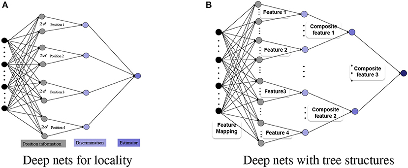
Figure 3. Deep nets with tree structures. (A) Deep nets for locality. (B) Deep nets with tree structures.

It is important to emphasize that the aim of the present paper is not to pursue the advantages of deep nets with tree structures in approximation, since this has been the subject of investigation in a vast amount of literature (see for example [6, 9, 10, 13, 15, 17, 26]), but to show the benefit of tree structures in deriving small variance. In particular, using the tree structures, we are able to decouple deep nets, layer by layer, and derive a tight covering number [27] estimate by using the Lipschitz property of the activation function. Since there are much fewer free parameters in deep nets with tree structures than those in DFCN, with the same number of neurons, the covering number of the former is smaller than that of the latter, resulting in smaller variance of deep nets with tree structures. We will then derive fast learning rates for “generalization error” for implementing the empirical risk minimization on deep nets. Deep nets with tree structures, revealed by our study, possess three theoretical advantages, namely: the capacity, as measured by the covering number, is much smaller than that of DFCN; based on tree structures, the approximation capability is comparable with that of DFCN; and fast learning rate is achieved, by applying an empirical risk minimization algorithm.

2. Deep Nets With Tree Structures

In image processing, a standard approach is to leverage a low-dimensional image to a high-dimensional pixel-scale image. While leveraging is a brutal approach that loses such image features as sparsity, locality and symmetry, and makes the variables highly inter-related, one method to capture the structure information by means of grouping the adjacent variables is machine learning. In particular, DCNN with numerous hidden layers, as exhibited in Figure 4, has been utilized, with the underlying intuition that the convolutional structure can extract missing features by deepening the network. The problem is, however, that with the exception of being able to extract transition-invariance features [28], there is no theoretical verification that DCNN could out-perform other neural network structures in feature extraction. Motivated by the application of DCNN in image processing, we propose a novel structure to equip deep nets for feature extraction and learning. Our basic idea is to group different features via several neurons in the first hidden layer rather than brutal leveraging. In this way, each group is independent and thus a tree structure feature extraction is sufficient to extract the grouped feature, just as Figure 3B purports to show.

FIGURE 4

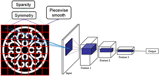
Figure 4. DCNN in image processing.

In the following, we present the detailed definition of deep nets with tree structures. Let 𝕀: = [−1, 1], x = (x⁽¹⁾, …, x^(d)) ∈ 𝕀^d = [−1, 1]^d, and L ∈ ℕ denote the number of hidden layers. Also let ϕ_k : ℝ → ℝ, k = 0, 1, …, L, be univariate activation functions. Let N₀ = d and for each j = 1, …, L, denote by N_j ≥ 2, the size of tree in the j-th hidden layer. Set

$\begin{array}{l}{H}_{{\overrightarrow{\alpha }}_0,0}(\text{x})={\displaystyle \sum _{j=1}^{N_0}}{a}_{j,{\overrightarrow{\alpha }}_0,0}{\varphi }_0(w_{j,{\overrightarrow{\alpha }}_0,0}{x}^{(j)}+b_{j,{\overrightarrow{\alpha }}_0,0}),\\ \text{x}=(x^{(1)},\dots ,x^{(d)}),{\overrightarrow{\alpha }}_0\in {\displaystyle \prod _{i=1}^L}\left\{1,2,\dots ,N_i\right\}.& (1)\end{array}$

Then a deep net with the tree structure of L layers can be formulated recursively by

$\begin{array}{l}{H}_{{\overrightarrow{\alpha }}_k,k}(\text{x})={\displaystyle \sum _{j=1}^{N_k}}{a}_{j,{\overrightarrow{\alpha }}_k,k}{\varphi }_k(H_{j,{\overrightarrow{\alpha }}_k,k-1}(\text{x})+b_{j,{\overrightarrow{\alpha }}_k,k}),\\ 1\le k\le L,{\overrightarrow{\alpha }}_k\in {\displaystyle \prod _{i=k+1}^L}\left\{1,2,\dots ,N_i\right\},& (2)\end{array}$

where $a_{j,{\overrightarrow{\alpha }}_k,k},b_{j,{\overrightarrow{\alpha }}_k,k},w_{j,{\overrightarrow{\alpha }}_0,0}\in ℝ$ for each j ∈ {1, 2, …, N_k}, k ∈ {0, 1, …, L}, ${\prod }_{L+1}^L\left\{1,2,\dots ,N_L\right\}=\varnothing$ and $H_{{\overrightarrow{\alpha }}_{k-1},k-1}(x)=(H_{1,\overrightarrow{{\alpha }_k},k-1}(x),\dots ,H_{N_k,\overrightarrow{{\alpha }_k},k-1}(x))$. Let ${{H}}_L^{tree}$ denote the set of output functions $H_L=H_{{\overrightarrow{\alpha }}_L,L}$ for ${\overrightarrow{\alpha }}_L\in \varnothing$ at the L-th layer. For 0 ≤ k ≤ L − 1 and ${\overrightarrow{\alpha }}_k\in {\prod }_{i=k+1}^L\left\{1,2,\dots ,N_i\right\}$, denote by ${{H}}_{{\overrightarrow{\alpha }}_k,k}^{tree}$ the set of functions $H_{{\overrightarrow{\alpha }}_k,k}$ defined in (2).

By setting ϕ₀(t) = t and $b_{j,{\overrightarrow{\alpha }}_0,0}=0$, it is easy to see that ${{H}}_1^{tree}$ reduces to the classical shallow net. In view of the tree structure, it follows from (1), (2) and Figure 5 that there are a total of

$\begin{array}{ll}{{A}}_L:=2{\displaystyle \sum _{k=0}^L}{\Pi }_{\ell =0}^{L-k}{N}_{L-\ell }+{\Pi }_{\ell =0}^L{N}_{\ell }& (3)\end{array}$

free parameters for $H_L\in {{H}}_L^{tree}$. For $\alpha ,{R}\ge 1$, we introduce the notation

$\begin{array}{ll}{{H}}_{L,\alpha ,{R}}^{tree}& :=\{H_L\in {{H}}_L^{tree}:|a_{j,{\overrightarrow{\alpha }}_k,k}|,|b_{j,{\overrightarrow{\alpha }}_k,k}|,|w_{j,{\overrightarrow{\alpha }}_k,0}|\le {R}{({{A}}_L)}^{\alpha },\\ & 0\le k\le L,1\le j\le N_k,{\overrightarrow{\alpha }}_k\in {\displaystyle \prod _{i=k+1}^L}\{1,2,\dots ,N_i\}\}.& (4)\end{array}$

With the restrictions imposed by (4) on deep nets, the parameters are bounded. This is indeed a necessity condition, since it can be found in Guo et al. [29] and Maiorov and Pinkus [15] that there exists some $h\in {{H}}_{2,\infty ,\infty }^{tree}$ with finitely many neurons but infinite capacity (covering number).

FIGURE 5

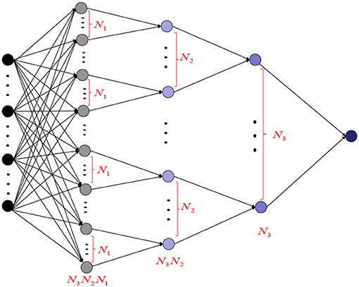
Figure 5. Size of tree in deep nets.

3. Advantages of Deep Nets With Tree Structures

The study of the advantages of deep nets over shallow nets in approximation is a classical topic and several theoretical benefits of deep nets are revealed in a large literature. We refer the readers to a fruitful review paper [18] for more details. Due to the concise mathematical formulation, deep nets with tree structures are one of the most popular structures in approximation theory. It dates back to Mhaskar [26], where it was proved that deep nets with tree structures can be constructed to overcome the saturation phenomenon of shallow nets in the sense that the approximation rate cannot go beyond a certain level when the regularity of the target function increases. In Chui et al. [6], deep nets with two hidden layers and tree structures were constructed to provide localized approximation, which is beyond the performance of shallow nets. In Maiorov and Pinkus [15], a deep net with tree structures, two hidden layers and finitely many neurons, was demonstrated to possess the universal approximation property. Furthermore, in our recent papers Chui et al. [10, 17], deep nets with tree structures were proved to be capable of extracting the manifold structure feature and rotation-invariance feature, respectively.

Most importantly, it is clear from the above-mentioned results that deep nets with tree structures do not degrade the approximation performance of DFCN, while sparse connections between neurons significantly reduces the number of free parameters. In the following, we will show that deep nets with tree structures have an overall advantage over DFCN by deriving tight covering number estimates. Let 𝔹 be a Banach space and V be a subset of 𝔹. Denote by ${N}(\epsilon ,V,B)$ the ε-covering number of V under the metric of 𝔹 [27], defined by the minimal number of elements in an ε-net of V. For $𝔹=L_{\infty }(I^d)$, we set ${N}(\epsilon ,V):={N}(\epsilon ,V,L_{\infty }({𝕀}^d))$ for brevity. The objective of this consideration is to establish the following theorem, that exhibits a tight bound for covering numbers of ${{H}}_{L,\alpha ,{R}}^{tree}$.

Theorem 1. Assume that

$\begin{array}{l}\hfill |{\varphi }_j(t)-{\varphi }_j(t^{\prime })|\le c_1|t-t^{\prime }|,and\left|{\varphi }_j(t)\right|\le 1,\hfill \\ \hfill \forall t,t^{\prime }\in ℝ,j=0,\dots ,L.\hfill & (5)\end{array}$

Then for any 0 < ε ≤ 1,

$\begin{array}{ll}{N}(\epsilon ,{{H}}_{L,\alpha ,{R}}^{tree})\le {\left(\frac{2^{L+5/2}{c}_1^{L+3/2}{{A}}_{R,\alpha ,L}^{L+1}}{\epsilon }\right)}^{2{{A}}_L},& (6)\end{array}$

where ${{A}}_{R,\alpha ,L}:={R}{({{A}}_L)}^{\alpha }$ and ${{A}}_L$ is defined by (3).

The proof of Theorem 1 is delayed to section 5. We remark that the assumption (5) is mild. Indeed, almost all widely used activation functions including the logistic function $\varphi (t)=\frac{1}{1+e^{-t}}$, hyperbolic tangent sigmoidal function $\varphi (t)=\frac{1}{2}(\text{tanh}(t)+1)$ with tanh(t) = (e^2t − 1)/(e^2t + 1), arctan sigmoidal function $\varphi (t)=\frac{1}{\pi }\text{arctan}(t)+\frac{1}{2},$ Gompertz function ϕ(t) = e^−ae−bt with a, b > 0 and Gaussian function σ(t) = e^−t2 satisfy this assumption. We also remark that numerous quantities such as the number of linear regions [20], Betti numbers [21], VC-dimension [30], and number of monomials [22] have been employed to measuring the capacity of deep nets. To compare these measurements, it is noted that covering numbers possess three advantages. Firstly, the covering number is close to the coding length in information theory according to the encode-decode theory proposed by Donoho [31]. Thus, it is a powerful capacity measurement to show the expressivity of deep nets. Secondly, covering numbers determine the limitations of approximation ability of deep nets [17, 29]. Therefore, studying covering numbers of deep nets facilitates the verification of the optimality of the existing approximation results in Chui et al. [6, 10, 17] and Mhaskar [26]. Finally, covering numbers usually correspond to some oracle inequalities [23] and can reflect the stability of learning algorithms. All these features suggest the rationality of adopting the covering number to measure the capacity of deep nets.

Under the Lipchitz assumption (5) for the activation function, a bound of the covering number for the set

$\begin{array}{l}{F}:=\{f=\sigma (w·\text{x}+b):w\in {ℝ}^d,b\in ℝ,{\Vert f\Vert }_{*}\le 1\}\end{array}$

with ‖ · ‖_* denoting some norm including the uniform norm was derived in Kůrková and Sanguineti [32]. Based on this, Maiorov [33] presented a tight estimate for shallow nets as

$\begin{array}{ll}{N}(\epsilon ,S_{\sigma ,n}^{*})={O}\left(n^d\text{ log}\frac{{\Gamma }_n}{\epsilon }\right),& (7)\end{array}$

where

$\begin{array}{lll}{S}_{\sigma ,n}^{*}:& =& \{{\displaystyle \sum _{j=1}^n}{c}_j\sigma (w_j·\text{x}+{\theta }_j):|c_j|,|w_j^{(i)}|,|{\theta }_j|\le {\Gamma }_n,\\ & & 1\le j\le n,1\le i\le d\}\end{array}$

and Γ_n > 0 depending on n.

Estimates of covering number for deep nets were first studied in Kohler and Krzyżak [34], where a tight bound for covering numbers of deep nets with tree structures and two hidden layers is derived. Using a similar approach, it was presented in Kohler and Krzyżak [34] and Lin [9] an upper bound estimate for deep nets with tree structures, five hidden layers and without the Liptchitz assumption (5) of the activation function. Recently, Kohler and Krzyzak [13] provided an estimate for covering numbers of deep nets with L-hidden layers with L ∈ ℕ. Furthermore, covering numbers for deep nets with arbitrary structures and bounded parameters were deduced in Guo et al. [29]. Our result, exhibited in Theorem 1, establishes a covering number estimate for deep nets with arbitrarily many hidden layers and tree structures. This result improves the estimate in Guo et al. [29] by reducing the exponent of ${{A}}_{R,\alpha ,L}$ from L² to (L + 1), since ${{A}}_{R,\alpha ,L}>1$ is usually very large. The main tool in our analysis is to use the Liptchitz property of the activation function and boundedness of the free parameters to decouple the depth layer by layer due to tree structures. It should be mentioned that Theorem 1 also removes the monotonic increasing assumption on the activation function while exhibits a similar covering number estimate as Anthony and Bartlett [35, Theorem 14.5]. Due to the boundedness assumption (5), our result excludes the covering number estimate for deep nets with the widely used rectifier linear unit (ReLU). Using the technique in Guo et al. [29, Lemma 1], we can derive upper bound estimates of deep nets in different layers. But it leads to an additional power L on ${{A}}_{R,\alpha ,L}^{L+1}$ in (6), i.e., ${{A}}_{R,\alpha ,L}^{L^2+L}$. Thus, it requires a novel technique to derive the same covering number estimate for deep ReLU nets as Theorem 1. We leave it as a future work.

4. Generalization Error Estimates for Deep Nets

In this section, we present the generalization error estimates for empirical risk minimization on deep nets in the framework of learning theory [23]. In this framework, samples $D_m={\left\{({\text{x}}_i,y_i)\right\}}_{i=1}^m$ are assumed to be drawn independently according to the Borel probability measure ρ on $\sout{{Z}}={X}\times {Y}$ with ${X}={𝕀}^d$ and ${Y}\subseteq \left[-M,M\right]$ for some M > 0. The primary objective is to apply the regression function:

$\begin{array}{l}{f}_{\rho }(\text{x})={\displaystyle {\int }_{{Y}}}yd\rho (y|\text{x}),\text{x}\in {X}\end{array}$

which minimizes the generalization error

$\begin{array}{l}\epsilon (f):={\displaystyle {\int }_{\sout{{Z}}}}{(f(\text{x})-y)}^{2}d\rho ,\end{array}$

where ρ(y|x) denotes the conditional distribution at x induced by ρ. Let ρ_X be the marginal distribution of ρ on ${X}$ and $\left(L_{{\rho }_X}^2,{\Vert \cdot \Vert }_{\rho }\right)$ be the Hilbert space of ρ_X square-integrable functions on ${X}$. For $f\in L_{{\rho }_X}^2$, we have [23]

$\begin{array}{ll}\epsilon (f)-\epsilon (f_{\rho })={\Vert f-f_{\rho }\Vert }_{\rho }^2.& (8)\end{array}$

Denote by ${\epsilon }_D(f):=\frac{1}{m}\sum _{i=1}^m{(f({\text{x}}_i)-y_i)}^2$ the empirical risk for the estimator f. Before presenting the generalization error for deep nets with tree structures, we derive an oracle inequality based on covering numbers for the empirical risk minimization (ERM) algorithm, i.e.,

$\begin{array}{ll}{f}_{D,{H}}=\text{arg }{\displaystyle \underset{f\in {H}}{\text{min }}}{\epsilon }_D(f),& (9)\end{array}$

where ${H}$ is a set of continuous functions on ${X}$ and is ${{H}}_{L,\alpha ,{R}}^{tree}$ in our study. Since |y| ≤ M almost everywhere, we have |f_ρ(x)| ≤ M. It is natural to project an output function $f:{X}\to ℝ$ onto the interval [−M, M] by the projection operator

$\begin{array}{l}{\pi }_{M}f(\text{x}):=\{\begin{array}{cc}f(\text{x}),\hfill & \text{if}-M\le f(\text{x})\le M,\hfill \\ M,\hfill & \text{if}f(\text{x})>M,\hfill \\ -M,\hfill & \text{if}f(\text{x})<-M.\hfill \end{array}\end{array}$

Thus, the estimator we study in this paper is ${\pi }_M{f}_{D,{H}}$. The following theorem presents the oracle inequality for ERM based on covering numbers.

Theorem 2. Suppose there exist $n^{\prime },{U}>0$, such that

$\begin{array}{ll}\text{log}{N}(\epsilon ,{H})\le n^{\prime }\text{log}\frac{{U}}{\epsilon },\forall \epsilon >0.& (10)\end{array}$

Then for any $h\in {H}$ and ϵ > 0,

$\begin{array}{l}Prob\{\Vert \pi M{f}_{D,{H}}-f_{\rho }{\Vert }_{\rho }^2>\epsilon +2\Vert h-f_{\rho }{\Vert }_{\rho }^2\}\\ \le \exp \left\{n^{\prime }\log \frac{16{U}M}{\epsilon }-\frac{3m\epsilon }{512M^2}\right\}\\ +\exp \left\{\frac{-3m{\epsilon }^2}{16{(3M+\Vert h{\Vert }_{L_{\infty }({X})})}^2\left(6\Vert h-f_{\rho }{\Vert }_{\rho }^2+\epsilon \right)}\right\}.\end{array}$

The proof of Theorem 2 will be given in the next section. Theorem 2 shows that the covering number plays an important role in deducing the generalization error. As a result of this theorem and Theorem 1, we can derive tight generalization error bounds for ERM on deep nets with tree structures. Suppose that there exist some β > 0, $\tilde{c}>0$, ${R}>0$ and α > 0, such that

$\begin{array}{ll}{\displaystyle \underset{g\in {{H}}_{L,\alpha ,{R}}^{tree}}{\text{min}}}\Vert f_{\rho }-g{\Vert }_{L^{\infty }({Ⅱ}^d)}\le \stackrel{\text{~}}{c}{{A}}_L^{-\beta }.& (11)\end{array}$

Define

$\begin{array}{ll}{f}_{D,L}=\text{arg}{\displaystyle \underset{f\in {{H}}_{L,\alpha ,{R}}^{tree}}{\text{min}}}{\epsilon }_D(f).& (12)\end{array}$

We then derive the following generalization error estimate for (12).

Theorem 3. Let 0 < δ < 1. Suppose that there exist some $\beta ,\tilde{c},\alpha ,{R}>0$ such that (11) holds. If (5) holds and $C^{\prime }{m}^{1/(2\beta +1)}\le L{A}_L\le C^{″}{m}^{1/(2\beta +1)}$, then with confidence at least 1 − δ, we have

$\begin{array}{ll}\epsilon ({\pi }_M{f}_{D,L})-\epsilon (f_{\rho })\le C{L}^{2\beta }{m}^{-\frac{2\beta }{2\beta +1}}\text{ log }m\text{ log }\frac{3}{\delta },& (13)\end{array}$

where C, C′, C″ are constants independent of ${{A}}_L$, L, N₁, …, N_L, m, or δ.

The proof of Theorem 3 will be given in the next section. Assumption (11) describes the expressivity of ${{H}}_{L,\alpha ,{R}}^{tree}$. For some constants $\alpha ,{R}$, the exponent β in (11) implies the regularity for the regression function f_ρ. In particular, it can be found in Chui et al. [17] and Guo et al. [29] that the Liptchitz continuity and radial property of f_ρ corresponds to β = 1/d and β = 1, respectively. It was shown in (13) that there is an additional L^2β in our estimate, which is different from generalization errors of shallow nets [36] and deep nets with fixed depth [10]. The main reason is that there is an additional L in the exponent for the covering numbers of ${{H}}_{L,\alpha ,{R}}^{tree}$ in (6). With the same number of parameters, large depth of deep nets with tree structures usually leads to large variance, as shown in (13). However, it was also shown in Chui et al. [6, 10, 17], Guo et al. [29], Lin [9, 37], Mhaskar and Poggio [12], and Pinkus [18] that the depth is necessary in improving the performance of deep nets. It would be of some interest to study the smallest depth of deep nets with tree structures in extracting specific features. This study is left in a future work.

5. Proofs of Main Results

To facilitate our proof of Theorem 1, let us first establish the following lemma:

Lemma 1. Let ι ∈ ℕ, 𝔸 ⊆ ℝ^ι, B be a Banach space of functions on 𝔸 and ${{R}}_1,{{R}}_2>0$. For ${F},{G}\subseteq B$, set ${F}\oplus {G}:=\left\{f+f^{*}:f\in {F},f^{*}\in {G}\right\}$ and ${F}\odot {G}:=\left\{f·f^{*}:f\in {F},f^{*}\in {G}\right\}$. Then it follows that for any ε, ν > 0,

$\begin{array}{ll}{N}(\epsilon +\nu ,{F}\oplus {G},B)\le {N}(\epsilon ,{F},B){N}(\nu ,{G},B).& (14)\end{array}$

In addition, if $\underset{x\in 𝔸}{max}\left|f(x)\right|\le {{R}}_1$, $\underset{x\in 𝔸}{max}\left|f^{*}(x)\right|\le {{R}}_2$ for all $f\in {F}$ and $f^{*}\in {G}$, and ${F}\odot {G}\subseteq B$, then

$\begin{array}{ll}{N}(\epsilon +\nu ,{F}\odot {G},B)\le {N}(\epsilon /{{R}}_2,{F},B){N}(\nu /{{R}}_1,{G},B).& (15)\end{array}$

Proof. Let {f₁, …, f_N} and $\left\{f_1^{*},\dots ,f_{N^{\prime }}^{*}\right\}$ be an ε-cover and a ν-cover of ${F}$ and ${G}$ with

$\begin{array}{ll}N={N}(\epsilon ,{F},B),\text{and}{N}^{\prime }={N}(\nu ,{G},B).& (16)\end{array}$

Then, for every $f\in {F}$ and $f^{*}\in {G}$, there exist k ∈ {1, …, N} and ℓ ∈ {1, …, N′}, such that

$\begin{array}{l}{\Vert f-f_k\Vert }_B<\epsilon ,{\Vert f^{*}-f_{\ell }^{*}\Vert }_B<\nu .\end{array}$

By the triangle inequality, we have

$\begin{array}{l}{\Vert f+f^{*}-f_k-f_{\ell }^{*}\Vert }_B{\le \Vert f-f_k\Vert }_B{+\Vert f^{*}-f_{\ell }^{*}\Vert }_B<\epsilon +\nu .\end{array}$

Thus, $\left\{f_k+f_{\ell }^{*}:1\le k\le N,1\le \ell \le N^{\prime }\right\}$ is an (ε + ν)-cover of ${F}\oplus {G}$. Therefore, (16) implies

$\begin{array}{l}{N}(\epsilon +\nu ,{F}\oplus {G},B)\le N{N}^{\prime }={N}(\epsilon ,{F},B){N}(\nu ,{G},B).\end{array}$

This establishes (14).

To prove (15), let {f₁, …, f_N*} and $\left\{f_1^{*},\dots ,f_{N_{*}^{\prime }}^{*}\right\}$ be an $\epsilon /{{R}}_2$-cover and a $\nu /{{R}}_1$-cover of ${F}$ and ${G}$, respectively, with

$\begin{array}{ll}{N}_{*}={N}(\epsilon /{{R}}_2,{F},B),\text{and}{N}_{*}^{\prime }={N}(\nu /{{R}}_1,{G},B).& (17)\end{array}$

Then, for every $f\in {F}$ and $f^{*}\in {G}$, there exist k ∈ {1, …, N_*} and $\ell \in \left\{1,\dots ,N_{*}^{\prime }\right\}$ that satisfy $\underset{x\in 𝔸}{max}\left|f_k(x)\right|\le {{R}}_1$ and $\underset{x\in 𝔸}{max}\left|f_{\ell }^{*}(x)\right|\le {{R}}_2$ such that

$\begin{array}{l}{\Vert f-f_k\Vert }_B<\epsilon /{{R}}_2,{\Vert f^{*}-f_{\ell }^{*}\Vert }_B<\nu /{{R}}_1.\end{array}$

It then follows from the triangle inequality that

$\begin{array}{l}{\Vert f·f^{*}-f_k·f_{\ell }^{*}\Vert }_B\le {\Vert f·f^{*}-f·f_{\ell }^{*}\Vert }_B+{\Vert f·f_{\ell }^{*}-f_k·f_{\ell }^{*}\Vert }_B\\ \le {{R}}_1{\Vert f^{*}-f_{\ell }^{*}\Vert }_B+{{R}}_2{\Vert f-f_k\Vert }_B<\nu +\epsilon ,\hfill \end{array}$

which implies that $\left\{f_k{f}_{\ell }^{*}:1\le k\le N_{*},1\le \ell \le N_{*}^{\prime }\right\}$ is an (ε + ν)-cover of ${F}\odot {G}$. This together with (17) imply

$\begin{array}{l}{N}(\epsilon +\nu ,{F}\odot {G},B)\le N_{*}{N}_{*}^{\prime }={N}(\epsilon /{{R}}_2,{F},B){N}(\nu /{{R}}_1,{G},B).\end{array}$

This completes the proof of Lemma 1.

We are now ready to prove Theorem 1 as follows.

Proof of Theorem 1: Define, for k ∈ {0, 1, …, L} and ${\overrightarrow{\alpha }}_k\in {\prod }_{i=k+1}^L\left\{1,2,\dots ,N_i\right\}$,

$\begin{array}{lll}{{H}}_{k,\alpha ,{R},L,{\overrightarrow{\alpha }}_k}^{tree}:& =& \{H_k\in {{H}}_{{\overrightarrow{\alpha }}_k,k}^{tree}:|a_{j,{\overrightarrow{\alpha }}_{\ell },\ell }|,|b_{j,{\overrightarrow{\alpha }}_{\ell },\ell }|,|w_{j,{\overrightarrow{\alpha }}_{\ell },0}|\le {{A}}_{R,\alpha ,L},\\ & & 0\le \ell \le k,1\le j\le N_{\ell },{\overrightarrow{\alpha }}_{\ell }\in {\displaystyle \prod _{i=\ell +1}^k}\{1,2,\dots ,N_i\}\}.\hfill & (18)\end{array}$

Then, (14) implies that for ε > 0,

$\begin{array}{ll}{N}(\epsilon ,{{H}}_{k,\alpha ,{R},L,{\overrightarrow{\alpha }}_k}^{tree})\le {\left({\displaystyle \underset{1\le j\le N_k}{\text{max}}}{N}(\epsilon /N_k,{{H}}_{k,j,\alpha ,{R},L,{\overrightarrow{\alpha }}_k}^{tree,*})\right)}^{N_k},& (19)\end{array}$

where for 1 ≤ j ≤ N_k,

$\begin{array}{l}{{H}}_{k,j,\alpha ,{R},L,\overrightarrow{\alpha }}^{tree,*}:=\{f_j^{*}(\text{x})=a_{j,{\overrightarrow{\alpha }}_k,k}{\varphi }_k(H_{\overrightarrow{\alpha },k-1}(\text{x})+b_{j,\overrightarrow{\alpha },\ell })\\ :\left|a_{j,{\overrightarrow{\alpha }}_{\ell },\ell }\right|,\left|b_{j,\overrightarrow{\alpha },\ell }\right|\le {{A}}_{R,\alpha ,L},\\ H_{j,{\overrightarrow{\alpha }}_{k-1},k-1}\in {{H}}_{k-1,\alpha ,{R},L,{\overrightarrow{\alpha }}_{k-1}}^{tree},\\ 0\le \ell \le k,{\overrightarrow{\alpha }}_{\ell }\in {\displaystyle \prod _{i=\ell +1}^k}\{1,2,\dots ,N_i\}\}.\end{array}$

For each j ∈ {1, …, N_k}, since $\left|a_{j,{\overrightarrow{\alpha }}_k,k}\right|\le {{A}}_{R,\alpha ,L}$ and ‖ϕ_k‖_L∞(ℝ) ≤ 1, we obtain, from (15) with ι = 1, B = L_∞(ℝ), ${{R}}_1={{A}}_{R,\alpha ,L}$ and ${{R}}_2=1$, that

$\begin{array}{l}{N}(\epsilon /N_k,{{H}}_{k,j_k,\alpha ,{R},L,{\overrightarrow{\alpha }}_k}^{tree,*})\le {N}(\epsilon /N_k,\{a_{j,{\overrightarrow{\alpha }}_k,k}:|a_{j,{\overrightarrow{\alpha }}_k,k}|\le {{A}}_{R,\alpha ,L}\})\\ {N}(\epsilon /(N_k{{A}}_{R,\alpha ,L}),{{H}}_{k,j,\alpha ,{R},L,{\overrightarrow{\alpha }}_k}^{tree,**}),& (20)\end{array}$

where

$\begin{array}{l}{{H}}_{k,j,\alpha ,{R},L,{\overrightarrow{\alpha }}_k}^{tree,**}:=\{f_j^{**}(\text{x})={\varphi }_k(H_{j,{\overrightarrow{\alpha }}_k,k-1}(\text{x})+b_{j,{\overrightarrow{\alpha }}_k,k}):\\ \left|b_{j,{\overrightarrow{\alpha }}_k,\ell }\right|\le {{A}}_{R,\alpha ,L},\\ H_{{\overrightarrow{\alpha }}_{k-1},k-1}\in {{H}}_{k-1,\alpha ,{R},L,{\overrightarrow{\alpha }}_{k-1}}^{tree},0\le \ell \le k-1,\\ {\overrightarrow{\alpha }}_{\ell }\in {\displaystyle \prod _{i=\ell +1}^{k-1}}\{1,2,\dots ,N_i\}\}.\end{array}$

Since ϕ_k satisfies (5), it follows from the definition of the covering number that

$\begin{array}{ll}{N}(\epsilon /N_k,\{a_{j,{\overrightarrow{\alpha }}_k,k}:|a_{j,{\overrightarrow{\alpha }}_k,k}|\le {{A}}_{R,\alpha ,L}\})\le \frac{2N_k{{A}}_{R,\alpha ,L}}{\epsilon }& (21)\end{array}$

and

$\begin{array}{l}{N}(\epsilon /(N_k{{A}}_{R,\alpha ,L}),{{H}}_{k,j,\alpha ,{R},L,{\overrightarrow{\alpha }}_k}^{tree,**})\le {N}(\epsilon /(c_1{N}_k{{A}}_{R,\alpha ,L}),\\ {{H}}_{k,j,\alpha ,{R},L,{\overrightarrow{\alpha }}_k}^{tree,***}),& (22)\end{array}$

where

$\begin{array}{l}{{H}}_{k,j,\alpha ,{R},L,\overrightarrow{\alpha }}^{tree,***}:=\{f_j^{***}(\text{x})=H_{{\overrightarrow{\alpha }}_{k-1},k-1}(\text{x})+b_{j,{\overrightarrow{\alpha }}_k,k}\\ :\left|b_{j,{\overrightarrow{\alpha }}_{\ell },\ell }\right|\le {{A}}_{R,\alpha ,L},\\ H_{j,{\overrightarrow{\alpha }}_{k-1},k-1}\in {{H}}_{k-1,\alpha ,{R},L,{\overrightarrow{\alpha }}_{k-1}}^{tree},0\le \ell \le k-1,\\ {\overrightarrow{\alpha }}_{\ell }\in {\displaystyle \prod _{i=\ell +1}^{k-1}}\{1,2,\dots ,N_i\}\}.\end{array}$

Using (14) again, we have

$\begin{array}{l}{N}(\epsilon /(c_1{N}_k{{A}}_{R,\alpha ,L}),{{H}}_{k,j,\alpha ,{R},L,{\overrightarrow{\alpha }}_k}^{tree,***})\\ \le {N}(\epsilon /(2c_1{N}_k{{A}}_{{R},\alpha ,L}),\{b_{j,{\overrightarrow{\alpha }}_k,k}:|b_{j,{\overrightarrow{\alpha }}_k,k}|\le {{A}}_{{R},\alpha ,L}\})\\ {N}(\epsilon /(2c_1{N}_k{{A}}_{R,\alpha ,L}),{{H}}_{k-1,\alpha ,{R},L,{\overrightarrow{\alpha }}_{k-1}}^{tree})\\ \le \frac{4c_1{N}_k{{A}}_{R,\alpha ,L}}{\epsilon }{N}(\epsilon /(2c_1{N}_k{{A}}_{R,\alpha ,L}),{{H}}_{k-1,\alpha ,{R},L,{\overrightarrow{\alpha }}_{k-1}}^{tree}).& (23)\end{array}$

Combing (19), (20), (21), (22), and (23), we get

$\begin{array}{l}{N}(\epsilon ,{{H}}_{k,\alpha ,ℛ,L,{\overrightarrow{\alpha }}_k}^{tree})\le {\left(\frac{8c_1{N}_k^2{{A}}_{R,\alpha ,L}^2}{{\epsilon }^2}\right)}^{N_k}\hfill \\ {\left({N}(\epsilon /(2c_1{N}_k{{A}}_{R,\alpha ,L}),{{H}}_{k-1,\alpha ,ℛ,L,{\overrightarrow{\alpha }}_{k-1}}^{tree}))\right)}^{N_k}.\hfill & (24)\end{array}$

Using (24), we have

$\begin{array}{l}{N}(\epsilon ,{{H}}_{L,\alpha ,{R},L,{\overrightarrow{\alpha }}_L}^{tree})\le {\left(\frac{8c_1{N}_L^2{{A}}_{R,\alpha ,L}^2}{{\epsilon }^2}\right)}^{N_L}\\ {\left[{N}\left(\frac{\epsilon }{2c_1{N}_L{{A}}_{R,\alpha ,L}},{{H}}_{L-1,\alpha ,{R},L,{\overrightarrow{\alpha }}_{L-1}}^{tree}\right)\right]}^{N_L}\\ \le {\left(\frac{8c_1{N}_L^2{{A}}_{R,\alpha ,L}^2}{{\epsilon }^2}\right)}^{N_L}{\left(\frac{8c_1{\left(2c_1\right)}^2{N}_{L-1}^2{N}_L^2{{A}}_{R,\alpha ,L}^4}{{\epsilon }^2}\right)}^{N_L{N}_{L-1}}\\ \times {\left[{N}\left(\frac{\epsilon }{{\left(2c_1\right)}^2{{A}}_{R,\alpha ,L}^2{N}_L{N}_{L-1}},{{H}}_{L-2,\alpha ,{R},L,{\overrightarrow{\alpha }}_{L-2}}^F\right)\right]}^{N_L{N}_{L-1}},\end{array}$

which implies by induction

$\begin{array}{ll}\hfill & {N}(\epsilon ,{{H}}_{L,\alpha ,ℛ,L,{\overrightarrow{\alpha }}_L}^{tree})\le {(2c_1)}^{2{\sum }_{k=1}^{L-1}(L-k){\prod }_{\ell =0}^{L-k}{N}_{L-\ell }}\hfill \\ \hfill \times & {({{A}}_{R,\alpha ,L})}^{2{\sum }_{k=1}^L(L-k+1){\prod }_{\ell =0}^{L-k}{N}_{L-\ell }}{\displaystyle \prod _{k=1}^L{\left({\displaystyle \prod _{\ell =k}^L{N}_{\ell }}\right)}^{2{\prod }_{\ell =k}^L{N}_{\ell }}}\hfill \\ \hfill & {\left(\frac{8c_1}{{\epsilon }^2}\right)}^{{\sum }_{k=1}^L{\prod }_{\ell =0}^{L-k}{N}_{L-\ell }}\hfill \\ \hfill \times & [{N}(\frac{\epsilon }{{(2c_1)}^L{{A}}_{R,\alpha ,L}^L{N}_L{N}_{L-1}{N}_{L-2}···N_1},\hfill \\ \hfill & {{{H}}_{0,\alpha ,ℛ,L,{\overrightarrow{\alpha }}_0}^{tree})]}^{N_L{N}_{L-1}{N}_{L-2}···N_1}.\hfill & (25)\end{array}$

For arbitrary ν > 0, using the same arguments as those in proving (24), we get

$\begin{array}{l}{N}(\nu ,{{H}}_{0,\alpha ,ℛ,L,{\overrightarrow{\alpha }}_0}^{tree})\le {\left(\frac{8c_1{N}_0^2{{A}}_{R,\alpha ,L}^2}{{\nu }^2}\right)}^{N_0}\hfill \\ \times (\underset{1\le j\le N}{\max }{N}(\nu /(2c_1{N}_0{{A}}_{R,\alpha ,L}),\{w_{j,{\overrightarrow{\alpha }}_0,0}{x}^{(j_0)}+b_{j,{\overrightarrow{\alpha }}_0,0}\hfill \\ {:|w_{j,{\overrightarrow{\alpha }}_0,0}|,|b_{j,{\overrightarrow{\alpha }}_0,0}|\le {{A}}_{R,\alpha ,L}\})))}^{N_0}.\hfill \end{array}$

For j ∈ {1, …, N₀} and $0\le x^{(j_0)}\le 1$, noting that $\left\{w_{j,{\overrightarrow{\alpha }}_0,k}{x}^{(j_0)}+b_{j,{\overrightarrow{\alpha }}_0,k}:|w_{j,{\overrightarrow{\alpha }}_0,0}|,|b_{j,{\overrightarrow{\alpha }}_0,0}|\le {{A}}_{R,\alpha ,L}\right\}$ is in a two dimensional linear space whose elements are bounded by $2{{A}}_{R,\alpha ,L}$, we get

$\begin{array}{l}{N}(\nu /(2c_1{N}_0{{A}}_{R,\alpha ,L}),\{w_{j,\overrightarrow{\alpha },0}{x}^{(j_0)}+b_{j,\overrightarrow{\alpha },0}:|w_{j,\overrightarrow{\alpha },0}|,|b_{j,\overrightarrow{\alpha },0}|\\ \le {{A}}_{R,\alpha ,L}\})\le {\left(\frac{8c_1{N}_0{{A}}_{R,\alpha ,L}^2}{\nu }\right)}^2.\end{array}$

This implies

$\begin{array}{l}{N}(\epsilon /({(2c_1)}^L{{A}}_{R,\alpha ,L}^L{N}_L{N}_{L-1}{N}_{L-2}···N_1),{{H}}_{0,\alpha ,{R},L,{\overrightarrow{\alpha }}_0}^{tree}))\\ \le {\left(\frac{8c_1{(2c_1)}^{2L}{{A}}_{R,\alpha ,L}^{2L+2}{N}_L^2{N}_{L-1}^2···N_0^2}{\epsilon }\right)}^{N_0}\\ {\left(\frac{8c_1{(2c_1)}^L{{A}}_{R,\alpha ,L}^{L+1}{N}_L{N}_{L-1}{N}_{L-2}···N_1{N}_0}{\epsilon }\right)}^{2N_0}.\end{array}$

Inserting this estimate into (25), we have

$\begin{array}{l}{N}(\epsilon ,{{H}}_{L,\alpha ,{R},L,{\overrightarrow{\alpha }}_0}^{tree})\le {(2c_1)}^{2{\sum }_{k=0}^{L-1}(L-k){\prod }_{\ell =0}^{L-k}{N}_{L-\ell }}\\ {({{A}}_{R,\alpha ,L})}^{2{\sum }_{k=0}^L(L-k+1){\prod }_{\ell =0}^{L-k}{N}_{L-\ell }}\\ \times {\displaystyle \prod _{k=0}^L}{\left({\displaystyle \prod _{\ell =k}^L}{N}_{\ell }\right)}^{2{\prod }_{\ell =k}^L{N}_{\ell }}{\left(\frac{8c_1}{{\epsilon }^2}\right)}^{{\sum }_{k=0}^L{\prod }_{\ell =0}^{L-k}{N}_{L-\ell }}\\ \times {\left(\frac{8c_1{(2c_1)}^L{{A}}_{R,\alpha ,L}^{L+1}{N}_L{N}_{L-1}{N}_{L-2}···N_1{N}_0}{\epsilon }\right)}^{2N_0{N}_1···N_L}.\end{array}$

Recalling (3), N_k ≥ 2 for arbitrary k ∈ {0, 1, …, N}, we have

$\begin{array}{l}2{\displaystyle \sum _{k=0}^L}(L-k+1){\displaystyle \prod _{\ell =0}^{L-k}}{N}_{L-\ell }+2(L+1){\displaystyle \prod _{\ell =0}^L}{N}_{\ell }\le 2(L+1){{A}}_L,\\ \hfill 2{\displaystyle \sum _{k=0}^L}{\displaystyle \prod _{\ell =0}^{L-k}}{N}_{L-\ell }+2{\displaystyle \prod _{\ell =0}^L}{N}_{\ell }\le 2{{A}}_L\end{array}$

and

$\begin{array}{l}\left[{\displaystyle \prod _{k=0}^L}{\left({\displaystyle \prod _{\ell =k}^L}{N}_{\ell }\right)}^{2{\prod }_{\ell =k}^L{N}_{\ell }}\right]\left[{\left({\displaystyle \prod _{k=0}^L}{N}_k\right)}^{2{\prod }_{k=0}^L{N}_k}\right]\\ \le \left[{\left({\displaystyle \prod _{k=0}^L}{N}_k\right)}^{\left(2L+4\right){\prod }_{k=0}^L{N}_k}\right]\le {{A}}_L^{\left(L+1\right){{A}}_L}.\end{array}$

Thus, ${{A}}_L\le {{A}}_{{R},\alpha ,L}$ yields

$\begin{array}{l}{N}(\epsilon ,{{H}}_{L,\alpha ,{R}}^{tree})={N}(\epsilon ,{{H}}_{L,\alpha ,{R},L,{\overrightarrow{\alpha }}_L}^{tree})\le {(2c_1{{A}}_{R,\alpha ,L})}^{(2L+2){{A}}_L}\\ {\left(\frac{2\sqrt{2c_1}}{\epsilon }\right)}^{2{{A}}_L}\\ ={\left(\frac{2\sqrt{2c_1}{(2c_1{{A}}_{R,\alpha ,L})}^{2L+2}}{\epsilon }\right)}^{2{{A}}_L}={\left(\frac{2^{L+5/2}{c}_1^{L+3/2}{{A}}_{R,\alpha ,L}^{L+1}}{\epsilon }\right)}^{2{{A}}_L}.\end{array}$

This completes the proof of Theorem 1.

The proof of Theorem 2 depends on the following two concentration inequalities, which can be found in Cucker and Zhou [23], Wu and Zhou [38], and Zhou and Jetter [39], respectively.

Lemma 2 (B-Inequality). Let ξ be a random variable in a probability space $\sout{{Z}}$ with mean E(ξ) and variance σ²(ξ) = σ². If |ξ(z) − E(ξ)| ≤ M_ξ for almost all $z\in \sout{{Z}}$, then for any ε > 0,

$\begin{array}{l}Prob\left\{\frac{1}{m}{\displaystyle \sum _{i=1}^m}\xi (z_i)-E(\xi )>\epsilon \right\}\le \text{exp}\left\{-\frac{m{\epsilon }^2}{2({\sigma }^2+\frac{1}{3}{M}_{\xi }\epsilon )}\right\}.\end{array}$

Lemma 3 (C-Inequality). Let ${G}$ be a set of continuous functions on $\sout{{Z}}$ such that, for some $B^{\prime }>0,\tilde{c}>0$, |f^* − E(f^*)| ≤ B′ almost surely and $E({(f^{*})}^2)\le \tilde{c}E(f^{*})$ for all $f^{*}\in {G}$. Then for every ε > 0,

$\begin{array}{l}Prob\left\{{\displaystyle \underset{f^{*}\in {G}}{\text{sup}}}\frac{E(f^{*})-\frac{1}{m}{\displaystyle {\sum }_{i=1}^m}{f}^{*}(z_i)}{\sqrt{E(f^{*})+\epsilon }}>\sqrt{\epsilon }\right\}\le {N}(\epsilon ,{G},L_{\infty }({X}))\\ \text{exp}\left\{-\frac{m\epsilon }{2\stackrel{\text{~}}{c}+\frac{2B^{\prime }}{3}}\right\}.\end{array}$

We now turn to the proof of Theorem 2.

Proof of Theorem 2: For $h\in {H}$, from (9) we have ${\epsilon }_D(f_{D,{H}})\le {\epsilon }_D(h)$, which together with ${\epsilon }_D({\pi }_M{f}_{D,{H}})\le {\epsilon }_D(f_{D,{H}})$, implies

$\begin{array}{l}\epsilon ({\pi }_M{f}_{D,{H}})-\epsilon (f_{\rho })\le \epsilon (h)-\epsilon (f_{\rho })+{\epsilon }_D(h)\\ -\epsilon (h)+\epsilon ({\pi }_M{f}_{D,{H}})-{\epsilon }_D({\pi }_M{f}_{D,{H}}).\end{array}$

In the following we set, for convenience,

$\begin{array}{lll}{D}({H}):& =& \epsilon (h)-\epsilon (f_{\rho })={\Vert h-f_{\rho }\Vert }_{\rho }^2,\\ S_1(m,{H}):& =& \{{\epsilon }_D(h)-{\epsilon }_D(f_{\rho })\}-\{\epsilon (h)-\epsilon (f_{\rho })\}\end{array}$

and

$\begin{array}{l}{S}_2(m,{H}):=\{\epsilon ({\pi }_M{f}_{D,{H}})-\epsilon (f_{\rho })\}-\{{\epsilon }_D({\pi }_M{f}_{D,{H}})-{\epsilon }_D(f_{\rho })\}.\end{array}$

Then we have

$\begin{array}{ll}\epsilon ({\pi }_M{f}_{D,{H}})-\epsilon (f_{\rho })\le {D}({H})+{{S}}_1(m,{H})+{{S}}_2(m,{H}).& (26)\end{array}$

To apply the B-Inequality in Lemma 2, let the random variable ξ on $\sout{{Z}}$ be defined by

$\begin{array}{l}\xi (z)={(y-h(x))}^2-{(y-f_{\rho }(x))}^2.\end{array}$

Then since |y| ≤ M and |f_ρ(x)| ≤ M almost surely, we have

$\begin{array}{l}\left|\xi (z)\right|\le M_{\xi }^{\prime }:={(3M+{\Vert h\Vert }_{L_{\infty }({X})})}^2,|\xi -E\xi |\le 2M_{\xi }^{\prime },\text{and}\\ {\sigma }^2\le E({\xi }^2)\le M_{\xi }^{\prime }{D}({H})\end{array}$

almost surely. It then follows from B-Inequality with $M_{\xi }=2M_{\xi }^{\prime }$, that

$\begin{array}{ll}{{S}}_1(D,{H})\le \epsilon & (27)\end{array}$

holds with confidence at least

$\begin{array}{l}1-\text{exp}\left\{-\frac{m{\epsilon }^2}{2({\sigma }^2+\frac{1}{3}{M}_{\xi }\epsilon )}\right\}\ge 1\\ -\text{exp}\left\{-\frac{m{\epsilon }^2}{2{(3M+{\Vert h\Vert }_{L_{\infty }({X})})}^2({D}({H})+\frac{2}{3}\epsilon )}\right\}.& (28)\end{array}$

On the other hand, for

$\begin{array}{l}{G}:=\{f^{*}={({\pi }_{M}f(x)-y)}^2-{(f_{\rho }(x)-y)}^2:f\in {H}\}.\end{array}$

and any (fixed) $f^{*}\in {G},$ there exists an $f\in {H}$ such that $f^{*}(z)={({\pi }_{M}f(x)-y)}^2-{(f_{\rho }(x)-y)}^2$. Therefore, it follows from (8) that

$\begin{array}{l}E(f^{*})=\epsilon ({\pi }_{M}f)-\epsilon (f_{\rho })={\Vert {\pi }_{M}f-f_{\rho }\Vert }_{\rho }^2,\\ \frac{1}{m}{\displaystyle \sum _{i=1}^m}{f}^{*}(z_i)={\epsilon }_D({\pi }_{M}f)-{\epsilon }_D(f_{\rho }),\end{array}$

and

$\begin{array}{l}{f}^{*}(z)=({\pi }_{M}f(x)-f_{\rho }(x))[({\pi }_{M}f(x)-y)+(f_{\rho }(x)-y)].\end{array}$

Since |y| ≤ M and |f_ρ(x)| ≤ M almost surely, we have

$\begin{array}{l}\left|f^{*}(z)\right|\le (M+M)(M+3M)\le 8M^2,\end{array}$

which implies

$\begin{array}{l}|f^{*}(z)-E(f^{*})|\le B^{\prime }:=16M^2,\text{and}\\ E({(f^{*})}^2)\le 16M^2{\Vert {\pi }_{M}f-f_{\rho }\Vert }_{\rho }^2=16M^{2}E(f^{*}).\end{array}$

Hence, we may apply C-Inequality to ${G}$, with $B^{\prime }=\tilde{c}=16M^2$, to conclude that

$\begin{array}{ll}{\displaystyle \underset{f\in {H}}{\text{sup}}}\frac{\epsilon ({\pi }_{M}f)-\epsilon (f_{\rho })-({\epsilon }_D({\pi }_{M}f)-{\epsilon }_D(f_{\rho }))}{\sqrt{\epsilon ({\pi }_{M}f)-\epsilon (f_{\rho })+\epsilon }}<\sqrt{\epsilon }& (29)\end{array}$

holds with confidence at least

$\begin{array}{l}1-{N}(\epsilon ,{G},L_{\infty }({X}\times {Y})\text{exp}\left\{-\frac{3m\epsilon }{128M^2}\right\}.\end{array}$

For any $f_1,f_2\in {H}$, we have

$\begin{array}{l}|{({\pi }_M{f}_1(x)-y)}^2-{({\pi }_M{f}_2(x)-y)}^2|\le 4M|{\pi }_M{f}_1(x)-{\pi }_M{f}_2(x)|\\ \le 4M|f_1(x)-f_2(x)|.\end{array}$

Thus, an $\frac{\epsilon }{4M}$-covering of ${H}$ provides an ε-covering of ${G}$ for any ε > 0. This implies that

$\begin{array}{l}{N}(\epsilon ,{G},L_{\infty }({X}\times {Y}))\le {N}(\epsilon /(4M),{H},L_{\infty }({X})).\end{array}$

This together with (10) implies

$\begin{array}{l}{N}(\epsilon ,{G},L_{\infty }({X}\times {Y}))\le \text{exp}\left\{n^{\prime }\text{log}\frac{4M{U}}{\epsilon }\right\}.\end{array}$

Hence, (29) implies that

$\begin{array}{ll}{{S}}_2(D,{H})\le \frac{1}{2}(\epsilon (f_{D,{H}})-\epsilon (f_{\rho }))+\epsilon & (30)\end{array}$

holds with confidence at least

$\begin{array}{ll}1-\text{exp}\left\{n^{\prime }\text{log}\frac{4M{U}}{\epsilon }-\frac{3m\epsilon }{128M^2}\right\}.& (31)\end{array}$

Inserting (27), (28), (30), and (31) into (26), we conclude that

$\begin{array}{l}\epsilon ({\pi }_M{f}_{D,{H}})-\epsilon (f_{\rho })\le 2{D}({H})+4\epsilon \end{array}$

holds with confidence at least

$\begin{array}{l}1-\text{exp}\left\{-\frac{m{\epsilon }^2}{2{(3M+{\Vert h\Vert }_{L_{\infty }({X})})}^2({D}({H})+\frac{2}{3}\epsilon )}\right\}\\ -\text{exp}\left\{n^{\prime }\text{log}\frac{4M{U}}{\epsilon }-\frac{3m\epsilon }{128M^2}\right\}.\end{array}$

This completes the proof of Theorem 2 by re-scaling 4ε to ε.

To complete the discussion in this paper, we now prove Theorem 3 by applying Theorem 1 and Theorem 2, as follows.

Proof of Theorem 3: Due to (11), there exists some $h\in {{H}}_{L,\alpha ,{R}}^{tree}$ such that

$\begin{array}{l}{\Vert f_{\rho }-h\Vert }_{\rho }^2\le {\tilde{c}}^2{{A}}_L^{-2\beta },{\Vert h\Vert }_{L^{\infty }(I^d)}\le M+\tilde{c}.\end{array}$

Since (5) holds, Theorem 1 implies

$\begin{array}{l}\text{log}{N}(\epsilon ,{{H}}_{L,\alpha ,{R}}^{tree})\le 2{{A}}_L(L+3)\text{log}\left(\frac{2c_1{{A}}_{R,\alpha ,L}}{\epsilon }\right).\end{array}$

Applying Theorem 2 with $n^{\prime }=2{{A}}_L(L+3)$, ${U}=2c_1{{A}}_{R,\alpha ,L}$ to ${{H}}_{L,\alpha ,{R}}^{tree}$ and setting $L{{A}}_L=\left[C_1^{*}{m}^{\frac{1}{2\beta +1}}\right]$ with $C_1^{*}$ giving below, we have that for

$\begin{array}{ll}\epsilon \ge 2{\tilde{c}}^2{{A}}_L^{-2\beta }\text{log}{{A}}_L\ge 2{\Vert h-f_{\rho }\Vert }_{\rho }^2,& (32)\end{array}$

so that

$\begin{array}{l}Prob\{{\Vert {\pi }_M{f}_{D,L}-f_{\rho }\Vert }_{\rho }^2>2\epsilon \}\le Prob\{{\Vert \pi }_M{f}_{D,L}\\ -f_{\rho }{\Vert }_{\rho }^2>\epsilon +2{\Vert h-f_{\rho }\Vert }_{\rho }^2\}\\ \le \text{exp}\left\{2{{A}}_L(L+3)\text{log}\frac{2c_1{{A}}_{R,\alpha ,L}}{\epsilon }-\frac{3m\epsilon }{512M^2}\right\}\\ +\text{exp}\left\{\frac{-3m{\epsilon }^2}{16{(4M+\stackrel{\text{~}}{c})}^2(6{\stackrel{\text{~}}{c}}^2{{A}}_L^{-2\beta }+\epsilon )}\right\}\\ \le \text{exp}\left\{{\stackrel{\text{~}}{c}}_{1}L{{A}}_L\text{log}{{A}}_L-\frac{3m\epsilon }{512M^2}\right\}+\text{exp}\left\{\frac{-3m\epsilon }{112{(4M+\stackrel{\text{~}}{c})}^2}\right\},\end{array}$

where ${\tilde{c}}_1$ is a constant independent of ${{A}}_L$ or L. Setting $C_1^{*}$ to be a constant independent of L or ${{A}}_L$ such that $L{{A}}_L=\left[C_1^{*}{m}^{\frac{1}{2\beta +1}}\right]$, $\epsilon \ge 2{\tilde{c}}^2{{A}}_L^{-2\beta }log{{A}}_L$ and ${\tilde{c}}_{1}L{{A}}_{L}log{{A}}_L\le \frac{3m\epsilon }{1024M^2}$, we have

$\begin{array}{l}Prob\{{\Vert {\pi }_M{f}_{D,L}-f_{\rho }\Vert }_{\rho }^2>2\epsilon \}\le \text{exp}\left\{-\frac{3m\epsilon }{1024M^2}\right\}\\ +\text{exp }\left\{-\frac{-3m\epsilon }{112{(4M+\stackrel{\text{~}}{c})}^2}\right\}\le 2\text{ exp }\left\{-\frac{3m\epsilon }{112{(4M+\stackrel{\text{~}}{c})}^2}\right\}\\ \le 3\text{ exp }\left\{-\frac{3m^{\frac{2\beta }{2\beta +1}}\epsilon }{112{(4M+\stackrel{\text{~}}{c})}^2\text{log}{{A}}_L}\right\},& (33)\end{array}$

Then setting

$\begin{array}{l}3\text{exp}\left\{-\frac{3m^{\frac{2\beta }{2\beta +1}}\epsilon }{112{(4M+\stackrel{\text{~}}{c})}^2\text{log}{{A}}_L}\right\}=\delta ,\end{array}$

we obtain

$\begin{array}{l}2{\tilde{c}}^2{{A}}_L^{-2\beta }\text{log}{{A}}_L\le \epsilon \le \frac{112}{3}{({(C_1^{*})}^{2\beta }4M+\stackrel{\text{~}}{c})}^2{L}^{2\beta }{m}^{-\frac{2\beta }{2\beta +1}}\\ \text{log}{{A}}_L\text{log}\frac{3}{\delta }.\end{array}$

Thus, it follows from (33) that with confidence of at least 1 − δ, we have

$\begin{array}{l}{\Vert {\pi }_M{f}_{D,L}-f_{\rho }\Vert }_{\rho }^2\le C_2^{*}{L}^{2\beta }{m}^{-\frac{2\beta }{2\beta +1}}\text{ log }m\text{ log }\frac{3}{\delta },\end{array}$

where $C_2^{*}:=\frac{112}{3}{({(C_1^{*})}^{2\beta }4M+\tilde{c})}^2$. This completes the proof of Theorem 3.

6. Conclusion

In this paper, we provided a novel tree structure to equip deep nets and studied its theoretical advantages. Our studied showed that deep nets with tree structure succeeded in reducing the free parameters of deep fully-connected nets without sacrificing their excellent approximation ability. Under this circumstance, implementing the well known empirical risk minimization on deep nets with tree structures yields fast learning rates.

Data Availability

All datasets generated and analyzed for this study are included in the manuscript and the supplementary files.

Author Contributions

All authors listed have made a substantial, direct and intellectual contribution to the work, and approved it for publication.

Funding

The research of CC was partially supported by Hong Kong Research Council [Grant Nos. 12300917 and 12303218] and Hong Kong Baptist University [Grant No. HKBU-RC-ICRS/16-17/03]. The research of S-BL was supported by the National Natural Science Foundation of China [Grant No. 61876133], and the research of D-XZ was partially supported by the Research Grant Council of Hong Kong [Project No. CityU 11306617].

Conflict of Interest Statement

The authors declare that the research was conducted in the absence of any commercial or financial relationships that could be construed as a potential conflict of interest.

References

1. Hinton GE, Osindero S, Teh YW. A fast learning algorithm for deep belief netws. Neural Comput. (2006) 18:1527–54. doi: 10.1162/neco.2006.18.7.1527

PubMed Abstract | CrossRef Full Text | Google Scholar

2. Krizhevsky A, Sutskever I, Hinton GE. Imagenet Classification With Deep Convolutional Neural Networks. Lake Tahoe (2012). 1097–105.

Google Scholar

3. Lee H, Pham P, Largman Y, Ng AY. Unsupervised feature learning for audio classification using convolutional deep belief networks. In: Neural Information Processing Systems. Vancouver, BC (2010). p. 469–77.

Google Scholar

4. Silver D, Huang A, Maddison CJ, Guez A, Sifre L, van den Driessche G, et al. Mastering the game of Go with deep neural networks and tree search. Nature. (2016) 529:484–9. doi: 10.1038/nature16961

PubMed Abstract | CrossRef Full Text | Google Scholar

5. Goodfellow I, Bengio Y, Courville A. Deep Learning. London, UK: MIT Press (2016).

Google Scholar

6. Chui CK, Li X, Mhaskar HN. Neural networks for localized approximation. Math Comput. (1994) 63:607–23. doi: 10.2307/2153285

CrossRef Full Text | Google Scholar

7. Lin HW, Tegmark M, Rolnick D. Why does deep and cheap learning works so well? J Stat Phys. (2017) 168:1223–47. doi: 10.1007/s10955-017-1836-5

CrossRef Full Text | Google Scholar

8. Schwab C, Zech J. Deep learning in high dimension: neural network expression rates for generalized polynomial chaos expansions in UQ. Anal Appl. (2018). doi: 10.1142/S0219530518500203

CrossRef Full Text | Google Scholar

9. Lin SB. Generalization and expressivity for deep nets. IEEE Trans Neural Netw Learn Syst. (2019) 30:1392–406. doi: 10.1109/TNNLS.2018.2868980

PubMed Abstract | CrossRef Full Text | Google Scholar

10. Chui CK, Lin SB, Zhou DX. Construction of neural networks for realization of localized deep learning. Front Appl Math Stat. (2018) 4:14. doi: 10.3389/fams.2018.00014

CrossRef Full Text | Google Scholar

11. Shaham U, Cloninger A, Coifman RR. Provable approximation properties for deep neural networks. Appl Comput Harmon Anal. (2018) 44:537–57. doi: 10.1016/j.acha.2016.04.003

CrossRef Full Text | Google Scholar

12. Mhaskar H, Poggio T. Deep vs shallow networks: an approximation theory perspective. Anal Appl. (2006) 14:829–48. doi: 10.1142/S0219530516400042

CrossRef Full Text | Google Scholar

13. Kohler M, Krzyzak A. Nonparametric regression based on hierarchical interaction models. IEEE Trans Inform Theory. (2017) 63:1620–30. doi: 10.1109/TIT.2016.2634401

CrossRef Full Text | Google Scholar

14. Petersen P, Voigtlaender F. Optimal aproximation of piecewise smooth functions using deep ReLU neural networks. Neural Netw. (2018) 108:296–330. doi: 10.1016/j.neunet.2018.08.019

PubMed Abstract | CrossRef Full Text | Google Scholar

15. Maiorov V, Pinkus A. Lower bounds for approximation by MLP neural networks. Neurocomputing. (1999) 25:81–91. doi: 10.1016/S0925-2312(98)00111-8

CrossRef Full Text | Google Scholar

16. Ismailov VE. On the approximation by neural networks with bounded number of neurons in hidden layers. J Math Anal Appl. (2014) 417:963–9. doi: 10.1016/j.jmaa.2014.03.092

CrossRef Full Text | Google Scholar

17. Chui CK, Lin SB, Zhou DX. Deep neural networks for rotation-invariance approximation and learning. Anal Appl. arXiv:1904.01814.

Google Scholar

18. Pinkus A. Approximation theory of the MLP model in neural networks. Acta Numer. (1999) 8:143–95. doi: 10.1017/S0962492900002919

CrossRef Full Text | Google Scholar

19. Poggio T, Mhaskar H, Rosasco L, Miranda B, Liao Q. Why and when can deep-but not shallow-networks avoid the curse of dimensionality: a review. Int J Auto Comput. (2017). 14: 503–19. doi: 10.1007/s11633-017-1054-2

CrossRef Full Text | Google Scholar

20. Montúfar G, Pascanu R, Cho K, Bengio Y. On the number of linear regions of deep neural networks. In: Neural Information Processing Systems. Montréal, QC (2014). p. 2924–32.

Google Scholar

21. Bianchini M, Scarselli F. On the complexity of neural network classifiers: a comparison between shallow and deep architectures, IEEE Trans Neural Netw Learn Syst. (2014) 25:1553–65. doi: 10.1109/TNNLS.2013.2293637

PubMed Abstract | CrossRef Full Text | Google Scholar

22. Delalleau O, Bengio Y. Shallow vs. deep sum-product networks. In: Advances in Neural Information Processing Systems. Granada (2011). p. 666–74.

Google Scholar

23. Cucker F, Zhou DX. Learning Theory: An Approximation Theory Viewpoint. Cambridge: Cambridge University Press (2007).

Google Scholar

24. Zhou DX. Deep distributed convolutional neural networks: universality. Anal Appl. (2018) 16:895–919. doi: 10.1142/S0219530518500124

CrossRef Full Text | Google Scholar

25. Zhou DX. Universality of deep convolutional neural networks. Appl Comput Harmonic Anal. arXiv:1805.10769.

Google Scholar

26. Mhaskar H. Approximation properties of a multilayered feedforward artificial neural network. Adv Comput Math. (1993) 1:61–80. doi: 10.1007/BF02070821

CrossRef Full Text | Google Scholar

27. Zhou DX. Capacity of reproducing kernel spaces in learning theory. IEEE Trans Inform Theory. (2003) 49:1743–52. doi: 10.1109/TIT.2003.813564

CrossRef Full Text | Google Scholar

28. Bruna J, Mallat S. Invariant scattering convolution networks. IEEE Trans Patt Anal Mach Intel. (2013) 35:1872–86. doi: 10.1109/TPAMI.2012.230

PubMed Abstract | CrossRef Full Text | Google Scholar

29. Guo ZC, Shi L, Lin SB. Realizing data features by deep nets. arXiv: 1901.00130.

Google Scholar

30. Harvey N, Liaw C, Mehrabian A. Nearly-tight VC-dimension bounds for piecewise linear neural networks. Conference on Learning Theory. Amsterdam (2017). p. 1064–8.

Google Scholar

31. Donoho DL. Unconditional bases are optimal bases for data compression and for statistical estimation. Appl Comput Harmonic Anal. (1993) 1:100–15. doi: 10.1006/acha.1993.1008

CrossRef Full Text | Google Scholar

32. Kůrková V, Sanguineti M. Estimates of covering numbers of convex sets with slowly decaying orthogonal subsets. Discrete Appl Math. (2007) 155:1930–42. doi: 10.1016/j.dam.2007.04.007

CrossRef Full Text | Google Scholar

33. Maiorov V. Pseudo-dimension and entropy of manifolds formed by affine-invariant dictionary. Adv Comput Math. (2006) 25:435–50. doi: 10.1007/s10444-004-7645-9

CrossRef Full Text | Google Scholar

34. Kohler M, Krzyżak A. Adaptive regression estimation with multilayer feedforward neural networks. J Nonparametric Stat. (2005) 17:891–913. doi: 10.1080/10485250500309608

CrossRef Full Text | Google Scholar

35. Anthony M, Bartlett PL. Neural Network Learning: Theoretical Foundations. Cambridge: Cambridge University Press (2009).

Google Scholar

36. Maiorov V. Approximation by neural networks and learning theory. J Complex. (2006) 22:102–17. doi: 10.1016/j.jco.2005.09.001

CrossRef Full Text | Google Scholar

37. Lin SB. Limitations of shallow nets approximation. Neural Netw. (2017) 94:96–102. doi: 10.1016/j.neunet.2017.06.016

PubMed Abstract | CrossRef Full Text | Google Scholar

38. Wu Q, Zhou DX. SVM soft margin classifiers: linear programming versus quadratic programming. Neural Comput. (2015) 17:1160–87. doi: 10.1162/0899766053491896

CrossRef Full Text | Google Scholar

39. Zhou DX, Jetter K. Approximation with polynomial kernels and SVM classifiers. Adv Comput Math. (2006) 25:323–44. doi: 10.1007/s10444-004-7206-2

CrossRef Full Text | Google Scholar