Stochastic AUC Optimization Algorithms With Linear Convergence

Area under the ROC curve (AUC) is a standard metric that is used to measure classification performance for imbalanced class data. Developing stochastic learning algorithms that maximize AUC over accuracy is of practical interest. However, AUC maximization presents a challenge since the learning objective function is defined over a pair of instances of opposite classes. Existing methods circumvent this issue but with high space and time complexity. From our previous work of redefining AUC optimization as a convex-concave saddle point problem, we propose a new stochastic batch learning algorithm for AUC maximization. The key difference from our previous work is that we assume that the underlying distribution of the data is uniform, and we develop a batch learning algorithm that is a stochastic primal-dual algorithm (SPDAM) that achieves a linear convergence rate. We establish the theoretical convergence of SPDAM with high probability and demonstrate its effectiveness on standard benchmark datasets.

1. Introduction

Quantifying machine learning performance is an important issue to consider when designing learning algorithms. Many existing algorithms maximize accuracy, however, it can be a misleading performance metric for several reasons. First, accuracy assumes that an equal misclassification cost for positive and negative labeling. This assumption is not viable for many real world examples such as medical diagnosis and fraud detection [1]. Also, optimizing accuracy is not suitable for important learning tasks such as imbalanced classification. To overcome these issues, Area Under the ROC Curve (AUC) [2, 3] is a standard metric for quantifying machine learning performance. It is used in many real world applications, such as ranking and anomaly detection. AUC concerns the overall performance of a functional family of classifiers and quantifies their ability of correctly ranking any positive instance with regards to a randomly chosen negative instance. This combined with the fact that AUC is not effected by imbalanced class data makes AUC a more robust metric than accuracy [4]. We will discuss maximizing AUC in a batch learning setting.

Learning algorithms that maximize AUC performance have been developed in both batch and online settings. Previously, most algorithms optimizing AUC for classification [5–8] were for batch learning, where we assume all training data is available making those methods not applicable to streaming data. However, online learning algorithms [9–14], have been proven to be very efficient to deal with large-scale datasets and streaming data. The issue with these studies is that they focus on optimizing the misclassification error or its surrogate loss. These works all attempt to overcome the problem that AUC is based on the sum of pairwise losses between examples from different classes, making the objective function quadratic in the number of samples. Overcoming this issue is the challenge of designing algorithms to optimize the AUC score in either setting.

In this work, we present a new stochastic batch learning algorithm for AUC maximization, SPDAM. The algorithm is based on our previous work that we can reformulate AUC maximization as a stochastic saddle point problem with the inclusion of a regularization term [15]. However, the key difference from our previous work is that SPDAM assumes that the distribution is uniform and is solved as a stochastic primal dual algorithm [16]. The proposed algorithm results in a faster convergence rate than existing state-of-the-art algorithms. When evaluating on several standard bench mark datasets, SPDAM achieves performances that are on par with other state-of-the-art AUC optimization methods with a significant improvement in running time.

The paper is organized as follows: Section 2 discusses related work. Section 3 briefly reformulates AUC optimization as a saddle point problem. Section 4 exploits section 3 with the assumption that the distribution is a uniform distribution over the data and introduces SPDAM. Section 5 details the experiments. Finally, section 6 gives some final thoughts.

2. Related Work

AUC has been studied extensively because it is an appropriate performance measure for when dealing with imbalanced data distributions for learning classification. Designing such algorithms that optimize AUC is a significant challenge because of the need for samples of opposite classes. An early work first maximized the AUC score directly by performing gradient descent constrained to a hypersphere [17]. Their algorithm used a differentiable approximation to the AUC score that was accurate and computationally efficient, being of the order of ${O}(n)$, where n is the number of data observations. Another early work optimized the AUC score using support vector machines [6].

In more recent work [18–22], significant progress has been done to design online learning algorithms for AUC maximization. Online methods are desirable for evaluating streaming data since these methods update when new data is available. However, a limitation of these methods is that the previous samples used need to be stored. For iteration t and where the dimension of the data is d, this results in a space and time complexity of ${O}(td)$. This is an undesirable property because these algorithms will not scale well for high-dimensional data as well as will require more resources. To overcome the quadratic nature of AUC, the problem of optimizing the AUC score can be reformulated as a sum of pairwise loss functions using hinge loss [19, 22]. The use of a buffer with size s was proposed. This lessens the complexity to ${O}(sd)$. However, if the buffer size is not set sufficiently large this will impact the performance of the method.

Again, using the idea of reformulating AUC as a sum of pairwise loss functions was further expanded upon [18]. Using the square loss function instead of hinge loss, a key observation was made in which the mean and covariance statistics of the training data could be easily updated as new data becomes available. Unlike the previous work where s samples needed to be stored, these statistics only needed to be stored. However, this algorithm still results in scaling issues for high-dimensional data because storing the covariance matrix results in a quadratic complexity of ${O}(d^2)$. The authors did make note of this issue and proposed using low-rank Gaussian matrices to approximate the covariance matrix. The approximation is not a general solution to the original problem and depends on whether the covariance matrix can be well approximated by low-rank matrices.

Work has been also been done to maximize AUC using batch methods. In Ding et al. [23], the authors propose an algorithm that uses an adaptive gradient method that uses the knowledge of historical gradients and that is less sensitive to parameter selection. The method proposed in Gultekin et al. [24] is based on a convex relaxation of the AUC function, but instead of using stochastic gradients, the algorithm uses the first and second order U-statistics of pairwise distances. A critical feature of this approach is that it is learning rate free as training the step size is a time consuming task.

More recently, work based on Ying et al. [25] has been expanded upon. The critical idea was the primal and dual variables introduced have distinct solutions. Two different works took advantage of this observation. The first work developed a primal dual style stochastic gradient method [26] while the other develops a stochastic proximal algorithm that can have non-smooth penalty functions [27, 28]. Both algorithms achieve a ${O}(1/T)$ convergence rate up to a logarithmic term.

3. Problem Statement

First, consider ${X}\subseteq {ℝ}^d$ to be the input space and ${Y}=\left\{-1,+1\right\}$ the output space. For the training data, z = {(x_i, y_i), i = 1, …, n}, we assume to be i.i.d. and the samples are obtained from an unknown distribution ρ on ${Z}={X}\times {Y}$. As in Ying et al. [25], we restrict this work to the family of linear functions, i.e., f(x) = w^⊤x.

3.1. AUC Optimization

The ROC curve is the plot of the true positive rate vs. the false positive rate. The area under the ROC curve (AUC) for any scoring function $f:{X}\to ℝ$ is equivalent to the probability of a positive sample ranking higher than a negative sample [3, 29]. It is defined as

$\begin{array}{ll}\text{AUC}(f)=Pr(f(x)\ge f(x^{\prime })|y=+1,y^{\prime }=-1),& (1)\end{array}$

where (x, y) and (x′, y′) are independently drawn from ρ. The intent of AUC maximization is to find the optimal decision function f:

$\begin{array}{l}arg{\displaystyle \underset{f}{max}}\text{AUC}(f)=arg{\displaystyle \underset{f}{min}}Pr(f(x)<f(x^{\prime })|y=1,y^{\prime }=-1)\\ =arg{\displaystyle \underset{f}{min}}E\left[I_{\left[f(x^{\prime })-f(x)>0\right]} |y=1,y^{\prime }=-1\right],& (2)\end{array}$

where 𝕀(·) is the indicator function. As in Ying et al. [25], define p = Pr(y = 1). Recall that the conditional expectation of a random variable ξ(z) is defined by $E\left[\xi (z)|y=1\right]=\frac{1}{p}\iint \xi (z)I_{y=1}d\rho (z)$. In (2), the indicator function is not continuous, and is usually replaced by a convex surrogate such as the ℓ₂ loss (1 − (f(x) − f(x′)))² or the hinge loss ${\left(1-(f(x)-f(x^{\prime }))\right)}_{+}$. We used the ℓ₂ loss for this work as it has been shown to be statistically consistent with AUC while the hinge loss is not [18, 30]. Letting λ be a regularization parameter, AUC maximization can be formulated by

$\begin{array}{ll}\begin{array}{c}{\displaystyle \underset{\text{w}}{argmin}}E\left[{(1-{\text{w}}^{\top }(x-x^{\prime }))}^2|y=1,y^{\prime }=-1\right]+\frac{\lambda }{2}{\Vert \text{w}\Vert }^2,\hfill \\ ={\displaystyle \underset{\text{w}}{argmin}}\frac{1}{p(1-p)}{{\displaystyle \iint }}_{{Z}\times {Z}}{(1-{\text{w}}^{\top }(x-x^{\prime }))}^2\hfill \\ I_{\left[y=1,y^{\prime }=-1\right]}d\rho (z)d\rho (z^{\prime })+\frac{\lambda }{2}{\Vert \text{w}\Vert }^2.\hfill \end{array}\hfill & (3)\end{array}$

where the samples (x, y) and (x′, y′) are independent. When ρ is a uniform distribution over training data z, we obtain the empirical minimization (ERM) problem for AUC optimization studied in Gao et al. [18] and Zhao et al. [22]

$\begin{array}{ll}{\displaystyle \underset{\text{w}}{argmin}}\frac{1}{n^{+}{n}^{-}}{\displaystyle \sum _{i=1}^n}{\displaystyle \sum _{j=1}^n}{(1-{\text{w}}^{\top }(x_i-x_j))}^2{I}_{[y_i=1\wedge y_j=-1]}+\frac{\lambda }{2}{\Vert \text{w}\Vert }^2,& (4)\end{array}$

where n⁺ and n⁻ denote the numbers of instances in the positive and negative classes, respectively.

3.2. Equivalent Representation as a Saddle Point Problem (SPP)

As in Ying et al. [25], AUC optimization as in (3) can be represented as stochastic Saddle Point Problem (SPP) (e.g., [15]). A stochastic SPP is generally in the form of

$\begin{array}{ll}{\displaystyle \underset{u\in {\Omega }_1}{min}}{\displaystyle \underset{\alpha \in {\Omega }_2}{max}}\left\{f(u,\alpha ):=E\left[F(u,\alpha ,\xi )\right]\right\},& (5)\end{array}$

where ${\Omega }_1\subseteq {ℝ}^d$ and ${\Omega }_2\subseteq {ℝ}^m$ are non-empty closed convex sets, ξ is a random vector with non-empty measurable set Ξ ⊆ ℝ^p, and F:Ω₁ × Ω₂ × Ξ → ℝ. Here $E\left[F(u,\alpha ,\xi )\right]={\int }_{\Xi }F(u,\alpha ,\xi )dPr(\xi )$, and function f(u, α) is convex in u ∈ Ω₁ and concave in α ∈ Ω₂. In general, u and α are referred to as the primal variable and the dual variable, respectively. In this work, we modified our formulation for AUC maximization to include a regularization term. We give a modified version of the result in Ying et al. [25] that includes the L² term. First, define $F:{ℝ}^d\times {ℝ}^3\times {Z}\to ℝ$, for any w ∈ ℝ^d, a, b, α ∈ ℝ and $z=(x,y)\in {Z}$, by

$\begin{array}{l}F(\text{w},a,b,\alpha ;z)=(1-p){({\text{w}}^{\top }x-a)}^2{I}_{\left[y=1\right]}+p{({\text{w}}^{\top }x-b)}^2{I}_{\left[y=-1\right]}\\ +2(1+\alpha )(p{\text{w}}^{\top }x{I}_{\left[y=-1\right]}-(1-p){\text{w}}^{\top }x{I}_{\left[y=1\right]})\\ -p(1-p){\alpha }^2+\frac{\lambda }{2}{\Vert \text{w}\Vert }^2.& (6)\end{array}$

Equation (6) is similar as in our previous work [25]. The only difference is the inclusion of a regularization term. The main result still holds in a similar manner.

Theorem 3.1. The AUC optimization (3) is equivalent to

$\begin{array}{ll}{\displaystyle \underset{\genfrac{}{}{0ex}{}{\text{w}\in {ℝ}^d}{(a,b)\in {ℝ}^2}}{min}}{\displaystyle \underset{\alpha \in ℝ}{max}}\left\{f(\text{w},a,b,\alpha ):={\displaystyle {\int }_{{Z}}}F(\text{w},a,b,\alpha ;z)d\rho (z)\right\}.& (7)\end{array}$

In addition, we can prove the following result.

Proposition 3.1. For any saddle point (w^*, a^*, b^*, α^*) of the SPP formulation (7), w^* is a minimizer of the original AUC optimization problem (3).

Proof: Let $\bar{f}(\text{w},a,b,\alpha )=1+\frac{{\int }_{{Z}}F(\text{w},a,b,\alpha ;z)d\rho (z)}{p(1-p)}+\frac{\lambda }{2}{\Vert \text{w}\Vert }^2$ and let (w^*, a^*, b^*, α^*) be a saddle point of the problem

$\begin{array}{l}{\displaystyle \underset{\genfrac{}{}{0ex}{}{\text{w}\in {ℝ}^d}{(a,b)\in {ℝ}^2}}{min}}{\displaystyle \underset{\alpha \in ℝ}{max}}\bar{f}(\text{w},a,b,\alpha ).\end{array}$

Since the order of the two minimization [i.e., minimizing with respect to w and minimizing with respect to (a, b) ] does not affect the result. This implies, for every fixed w, (a^*, b^*, α^*) is a saddle point of the sub-problem

$\begin{array}{l}{\displaystyle \underset{(a,b)\in {ℝ}^2}{min}}{\displaystyle \underset{\alpha \in ℝ}{max}}\bar{f}(\text{w},a,b,\alpha ).\end{array}$

Notice from the proof for Theorem 3.1 that

$\begin{array}{l}E\left[{(1-{\text{w}}^{\top }(x-x^{\prime }))}^2|y=1,y^{\prime }=-1\right]+\frac{\lambda }{2}{\Vert \text{w}\Vert }^2=\\ {\displaystyle \underset{(a,b)\in {ℝ}^2}{min}}{\displaystyle \underset{\alpha \in ℝ}{max}}\bar{f}(\text{w},a,b,\alpha ).& (8)\end{array}$

Hence,

$\begin{array}{l}E\left[{(1-{\text{w}}^{\top }(x-x^{\prime }))}^2|y=1,y^{\prime }=-1\right]+\frac{\lambda }{2}{\Vert \text{w}\Vert }^2=\bar{f}(\text{w},a^{*},b^{*},{\alpha }^{*}).\end{array}$

This further implies

$\begin{array}{l}{\displaystyle \underset{\text{w}}{min}}E\left[{(1-{\text{w}}^{\top }(x-x^{\prime }))}^2|y=1,y^{\prime }=-1\right]+\frac{\lambda }{2}{\Vert \text{w}\Vert }^2=\\ {\displaystyle \underset{\text{w}}{min}}f(\text{w},a^{*},b^{*},{\alpha }^{*}).& (9)\end{array}$

As w^* is a minimizer of the righthand side of the Equation (9), w^* is also a minimizer of the lefthand side of the equation.

4. Stochastic Primal-Dual Algorithm for AUC Maximization

The algorithm developed in our previous work focused on the population objective of the saddle point problem (7). It is essentially an online projected gradient descent algorithm which has an optimal convergence rate ${O}(1/\sqrt{t}).$ This convergence rate is distribution-free, i.e., it holds true for any distribution ρ.

In this section, we are concerned with the case that the distribution ρ in (7) is a uniform distribution over the given data z = {z₁, …, z_n}. Denote by ℕ_n = {1, 2, …, n} for any n ∈ ℕ. Now, when ρ is a uniform distribution over finite data {(x_i, y_i):i ∈ ℕ_n}, we can reformulate (4) as a SPP as in (5):

$\begin{array}{ll}{\displaystyle \underset{\genfrac{}{}{0ex}{}{\text{w}\in {ℝ}^d}{(a,b)\in {ℝ}^2}}{min}}{\displaystyle \underset{\alpha \in ℝ}{max}}\frac{1}{n}{\displaystyle \sum _{i\in {\mathbb{N}}_n}}F(\text{w},a,b,\alpha ,z_i).& (10)\end{array}$

In this case, the AUC optimization is equivalent to the saddle point problem (10). For this special case, we will develop in this section a stochastic primal-dual algorithm for AUC optimization (10) which is able to converge with a linear convergence rate. To this end, we now consider the following general saddle point problem for AUC maximization

$\begin{array}{l}{\displaystyle \underset{\text{w},a,b}{min}}{\displaystyle \underset{\alpha }{max}}\{\frac{1}{n_{+}}{\displaystyle \sum _{i\in {\mathbb{N}}_n}}{({\text{w}}^{\top }{x}_i-a)}^2{I}_{y_i=1}+\frac{1}{n_{-}}{\displaystyle \sum _{i\in {\mathbb{N}}_n}}{({\text{w}}^{\top }{x}_i-b)}^2{I}_{y_i=-1}\\ +2(1+\alpha ){\text{w}}^{\top }\left[\frac{1}{n_{-}}{\displaystyle \sum _{i\in {\mathbb{N}}_n}}{x}_i{I}_{y_i=-1}-\frac{1}{n_{+}}{\displaystyle \sum _{i\in {\mathbb{N}}_n}}{x}_i{I}_{y_i=1}\right]-{\alpha }^2\\ +\Omega (\text{w})\},& (11)\end{array}$

where Ω(w) is a penalty term. If Ω(w) = 𝕀_{‖w‖ ≤ R}(w), the above formulation is equivalent to the saddle point formulation (10).

Before describing the detailed algorithm, we introduce some notations and slightly modify the saddle formulation (11). Specifically, denote by n₊ and n₋ the numbers of samples in the positive and negative classes, respectively. In this discrete case $p=\frac{n_{+}}{n}.$ Let b = m₋ − m₊ where m₊ and m₋ are the means of the positive and negative classes, respectively, i.e., ${\text{m}}_{+}=\frac{1}{n_{+}}\sum _{i\in {\mathbb{N}}_n}{x}_i{I}_{y_i=1}$ and ${\text{m}}_{-}=\frac{1}{n_{-}}\sum _{i\in {\mathbb{N}}_n}{x}_i{I}_{y_i=-1}.$ For any i ∈ ℕ_n, denote

$\begin{array}{ll}{\bar{x}}_i=\frac{x_i-m_{+}}{\sqrt{2p}}\text{ if }{y}_i=1,{\bar{x}}_i=\frac{x_i-m_{-}}{\sqrt{2(1-p)}}\text{ if }{y}_i=-1.& (12)\end{array}$

Let $g(\text{w})=\frac{|{\text{b}}^{\top }\text{w}{|}^2}{2}+{\text{b}}^{\top }\text{w}+\Omega (\text{w}).$ To satisfy the hypothesis that g is a λ strong convex function, we will let $\Omega (\text{w})=\frac{\lambda }{2}{\Vert \text{w}\Vert }^2$. Now we have the following reformulation of (11), based on which we will develop a stochastic primal-dual algorithm for AUC maximization.

Proposition 4.1. Formulation (13) is equivalent to

$\begin{array}{ll}{\displaystyle \underset{\text{w}}{min}}{\displaystyle \underset{\beta }{max}}\left\{\frac{1}{n}{\displaystyle \sum _{i\in {\mathbb{N}}_n}}{\beta }_i{\text{w}}^{\top }{\bar{x}}_i-\frac{{\Vert \beta \Vert }^2}{2}+g(\text{w})\right\},& (13)\end{array}$

where g:ℝ^d → ℝ is defined, for any w ∈ ℝ^d, by $g(\text{w})=\frac{|{\text{b}}^{\top }\text{w}{|}^2}{2}+{\text{b}}^{\top }\text{w}+\Omega (\text{w}).$

Proof: By minimizing out a, b and α, formulation (11) is equivalent to

$\begin{array}{l}{\displaystyle \underset{\text{w}}{min}}{\displaystyle \underset{\alpha }{max}}\{\frac{1}{n_{+}}{\displaystyle \sum _{i\in {\mathbb{N}}_n}}{({\text{w}}^{\top }(x_i-{\text{m}}_{+}))}^2{I}_{y_i=1}\\ +\frac{1}{n_{-}}{\displaystyle \sum _{i\in {\mathbb{N}}_n}}{({\text{w}}^{\top }(x_i-{\text{m}}_{-}))}^2{I}_{y_i=-1}+2{\text{b}}^{\top }\text{w}+|{\text{b}}^{\top }\text{w}{|}^2+\Omega (\text{w})\}.\end{array}$

Substituting (12) into the above equation yields the desired result.

Recall that κ = max{‖x_i‖:i ∈ ℕ_n}. We can establish the following linear convergence rate of SPDAM.

Theorem 4.1. Assume that g is λ-strongly convex. Let (w^*, β^*) be the saddle point of (13). If the parameter σ, τ and θ are chosen such that

$\begin{array}{lll}\sigma & =& \frac{(n-m)+\sqrt{{(n-m)}^2+4n{\kappa }^{2}m/\lambda }}{8m{\kappa }^2},\tau =\frac{1}{4\sigma {\kappa }^2}and\\ \theta & =& 1-\frac{\lambda }{\lambda +2\sigma {\kappa }^2},\end{array}$

then, for any t ≥ 1, the SPDAM algorithm achieves

$\begin{array}{l}\left(\frac{1}{m}+\frac{1}{4\sigma m}\right)E\left[{\Vert {\beta }^{(t+1)}-{\beta }^{*}\Vert }^2\right]+\left(\lambda +\frac{1}{2\tau }\right)\hfill \\ E\left[\Vert {\text{w}}^{\left(t+1\right)}-{\text{w}}^{*}{\Vert }^2\right]+\frac{1}{4\tau }E\left[\Vert {\text{w}}^{(t+1)}-{\text{w}}^{(t)}{\Vert }^2\right]\hfill \\ \le {\theta }^t\left[\left(\frac{1}{m}+\frac{1}{2\sigma m}\right)\Vert {\beta }^{(0)}-{\beta }^{*}\Vert +\left(\lambda +\frac{1}{2\tau }\right)\Vert {\text{w}}^{(0)}-{\text{w}}^{*}{\Vert }^2\right].\hfill & (14)\end{array}$

Before we present the proof for the above theorem. It is useful to make some comments. Firstly, the proposed algorithm in Table 1 is inspired by the stochastic primal-dual algorithm proposed in Yu et al.[16] and Zhang and Lin [31] which focused on Support Vector Machines (SVM) and logistic regression. Secondly, the algorithm SPDAM enjoys faster convergence over the stochastic projected gradient method in our previous work. However, the incremental primal-dual algorithm here, in contrast to the algorithm in Table 1 which can deal with streaming data, is not an online learning algorithm, since it needs to know a priori the number of the samples, the ratio of the samples of positive class, and means of the positive and negative classes. We now will prove the main theorem. The following lemma is critical for proving Theorem 4.1.

TABLE 1

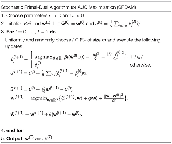
Table 1. Pseudo-code of Stochastic Primal-Dual Algorithm for AUC maximization.

Lemma 4.1. For the updates in SPDAM, we have

$\begin{array}{l}\left(\frac{1}{m}+\frac{1}{2\sigma m}\right)E\left[\Vert {\beta }^{(t+1)}-{\beta }^{*}{\Vert }^2\right]=\left(\frac{1}{2\sigma m}+\frac{n-m}{nm}\right)\\ E\left[\Vert {\beta }^{(t)}-{\beta }^{*}{\Vert }^2\right]-\frac{1}{2\sigma m}E\left[\Vert {\beta }^{(t+1)}-{\beta }^{(t)}{\Vert }^2\right]\\ +E\left[\langle {\overline{u}}^{(t+1)},{\bar{\text{w}}}^{(t)}-{\text{w}}^{*}\rangle \right],& (15)\end{array}$

and

$\begin{array}{l}\left(\lambda +\frac{1}{2\tau }\right)E\left[\Vert {\text{w}}^{(t+1)}-{\text{w}}^{*}{\Vert }^2\right]\le \frac{1}{2\tau }E\left[\Vert {\text{w}}^{(t)}-{\text{w}}^{*}{\Vert }^2\right]\\ -\frac{1}{2\tau }E\left[\Vert {\text{w}}^{(t+1)}-{\text{w}}^{(t)}{\Vert }^2\right]\\ -E\left[\langle {\overline{u}}^{(t+1)},{\text{w}}^{(t+1)}-{\text{w}}^{*}\rangle \right].& (16)\end{array}$

Proof: We first prove Equation (15). For any i ∈ ℕ_n, let ${\tilde{\beta }}_i$ be defined as

${\tilde{\beta }}_i=\underset{{\beta }_i\in ℝ}{\text{argmax}}\left\{{\beta }_i\langle {\bar{\text{w}}}^{(t)},x_i\rangle -\frac{|{\beta }_i{|}^2}{2}-\frac{|{\beta }_i-{\beta }_i^{(t)}{|}^2}{2\sigma }\right\}.$

Hence,

$\begin{array}{l}\frac{|{\beta }_i^{(t)}-{\beta }_i^{*}{|}^2}{2\sigma }+\frac{|{\beta }_i^{*}{|}^2}{2}-{\beta }_i^{*}\langle {\bar{\text{w}}}^{(t)},x_i\rangle =\frac{|{\beta }_i^{(t)}-{\tilde{\beta }}_i{|}^2}{2\sigma }+\frac{|{\tilde{\beta }}_i{|}^2}{2}\\ -{\tilde{\beta }}_i\langle {\bar{\text{w}}}^{(t)},x_i\rangle +\left(\frac{1}{2}+\frac{1}{2\sigma }\right)|{\tilde{\beta }}_i-{\beta }_i^{*}{|}^2.& (17)\end{array}$

Observe, by the definition of the saddle point (w^*, β^*), that

${\beta }^{*}=\underset{{\beta }_i}{\text{argmax}}\left\{{\beta }_i\langle {\text{w}}^{*},x_i\rangle -\frac{|{\beta }_i{|}^2}{2}\right\}.$

Consequently, ${\tilde{\beta }}_i\langle {\text{w}}^{*},x_i\rangle -\frac{|{\tilde{\beta }}_i{|}^2}{2}={\beta }_i^{*}\langle {\text{w}}^{*},x_i\rangle -\frac{|{\beta }_i^{*}{|}^2}{2}-\frac{1}{2}|{\tilde{\beta }}_i-{\beta }_i^{*}{|}^2$ which implies that $\frac{|{\tilde{\beta }}_i{|}^2}{2}-\frac{|{\beta }_i^{*}{|}^2}{2}=({\tilde{\beta }}_i-{\beta }_i^{*})\langle {\text{w}}^{*},x_i\rangle +\frac{1}{2}|{\tilde{\beta }}_i-{\beta }_i^{*}{|}^2.$ Putting this back into (17), we have

$\begin{array}{l}\frac{|{\beta }_i^{(t)}-{\beta }_i^{*}{|}^2}{2\sigma }+({\tilde{\beta }}_i-{\beta }_i^{*})\langle {\bar{\text{w}}}^{(t)}-{\text{w}}^{*},x_i\rangle =\frac{|{\beta }_i^{(t)}-{\tilde{\beta }}_i{|}^2}{2\sigma }\\ +\left(1+\frac{1}{2\sigma }\right)|{\tilde{\beta }}_i-{\beta }_i^{*}{|}^2.& (18)\end{array}$

Let ${{F}}_t$ be the sigma field generated by all random variables defined before round t. Taking expectation conditioned over ${{F}}_t$ implies that

$\begin{array}{l}E(|{\beta }_i^{(t)}-{\beta }_i^{(t+1)}{|}^2|{{F}}_t)=\frac{m}{n}|{\tilde{\beta }}_i-{\beta }_i^{(t)}{|}^2,\hfill \\ E(|{\beta }_i^{(t+1)}-{\beta }_i^{*}{|}^2|{{F}}_t)=\frac{m}{n}|{\tilde{\beta }}_i-{\beta }_i^{*}{|}^2+\frac{n-m}{n}|{\beta }_i^{(t)}-{\beta }_i^{*}{|}^2,\hfill \\ E(|{\beta }_i^{(t+1)}{|}^2|{{F}}_t)=\frac{m}{n}|{\tilde{\beta }}_i{|}^2+\frac{n-m}{n}|{\beta }_i^{(t)}{|}^2,\hfill \\ E({\beta }_i^{(t+1)}|{{F}}_t)=\frac{m}{n}{\tilde{\beta }}_i+\frac{n-m}{n}{\beta }_i^{(t)}.\hfill \end{array}$

Using the above equalities to represent terms involving ${\tilde{\beta }}_i$ by ${\beta }_i^{(t+1)}$ on the righthand side of (18), we have

$\begin{array}{l}\left(\frac{1}{m}+\frac{1}{2\sigma m}\right)E\left[|{\beta }_i^{(t+1)}-{\beta }_i^{*}{|}^2|{{F}}_t\right]=\left(\frac{1}{2\sigma m}+\frac{n-m}{nm}\right)\\ |{\beta }_i^{(t)}-{\beta }_i^{*}{|}^2-\frac{1}{2\sigma m}E[\Vert {\beta }^{(t+1)}-{\beta }^{(t)}{\Vert }^2]\\ +E\left[\langle {\bar{\text{w}}}^{(t)}-{\text{w}}^{*},\frac{1}{m}({\beta }_i^{t+1}-{\beta }_i^{*})+\frac{1}{n}({\beta }_i^{(t)}-{\beta }_i^{*})x_i\rangle |{{F}}_t\right]\end{array}$

Taking the summation over i ∈ ℕ_n and noticing that ${ū}^{(t+1)}=\frac{1}{m}\sum _{i\in {\mathbb{N}}_n}({\beta }_i^{t+1}-{\beta }_i^{*})x_i+\frac{1}{n}\sum _{i\in {\mathbb{N}}_n}({\beta }^{(t)}-{\beta }_i^{*})x_i$, we have

$\begin{array}{l}\left(\frac{1}{m}+\frac{1}{2\sigma m}\right)E\left[|{\beta }^{(t+1)}-{\beta }^{*}{|}^2|\right]=\left(\frac{1}{2\sigma m}+\frac{n-m}{nm}\right)\\ E[\Vert {\beta }^{(t)}-{\beta }^{*}{\Vert }^2]-\frac{1}{2\sigma m}E\left[\Vert {\beta }^{(t+1)}-{\beta }^{(t)}{\Vert }^2\right]\\ +E[\langle {\bar{\text{w}}}^{(t)}-{\text{w}}^{*},{\overline{u}}^{(t+1)}],\end{array}$

which completes the proof of the first estimation (15).

Now we turn our attention to the proof of inequality (16). Indeed, by the definition of w^(t+1) and λ-strongly convexity of g, there holds

$\begin{array}{l}\langle {\overline{u}}^{(t+1)},{\text{w}}^{*}\rangle +g({\text{w}}^{*})+\frac{\Vert {\text{w}}^{(t)}-{\text{w}}^{*}{\Vert }^2}{2\tau }\ge \langle {\overline{u}}^{(t+1)},{\text{w}}^{(t+1)}\rangle \\ +g({\text{w}}^{(t+1)})+\frac{\Vert {\text{w}}^{(t+1)}-{\text{w}}^{(t)}{\Vert }^2}{2\tau }\\ +\left(\frac{\lambda }{2}+\frac{1}{2\tau }\right)\Vert {\text{w}}^{(t+1)}-{\text{w}}^{*}{\Vert }^2.& (19)\end{array}$

Let $u^{*}=\frac{1}{n}\sum _{i\in {\mathbb{N}}_n}{\beta }_i^{*}{x}_i$. By the definition of the saddle point (w^*, β^*), there holds

$\begin{array}{l}\langle u^{*},{\text{w}}^{(t+1)}\rangle +g({\text{w}}^{(t+1)})\ge \langle u^{*},{\text{w}}^{*}\rangle +g({\text{w}}^{*})+\frac{\lambda }{2}\Vert {\text{w}}^{(t+1)}-{\text{w}}^{*}{\Vert }^2.\end{array}$

Adding the above inequality with (19) and arranging the terms yields that

$\begin{array}{l}\left(\lambda +\frac{1}{2\tau }\right)\Vert {\text{w}}^{(t+1)}-{\text{w}}^{*}{\Vert }^2\le \frac{\Vert {\text{w}}^{(t)}-{\text{w}}^{*}{\Vert }^2}{2\tau }-\frac{\Vert {\text{w}}^{(t+1)}-{\text{w}}^{(t)}{\Vert }^2}{2\tau }\\ -\langle {\text{w}}^{(t+1)}-{\text{w}}^{*},{\overline{u}}^{(t+1)}-u^{*}\rangle .\end{array}$

This completes the proof of the lemma.

Now we are ready to prove Theorem 4.1 using Lemma 4.1.

Proof: Adding (15) and (16) together, we have

$\begin{array}{l}\left(\frac{1}{m}+\frac{1}{2\sigma m}\right)E\left[\Vert {\beta }^{(t+1)}-{\beta }^{*}{\Vert }^2\right]+\left(\lambda +\frac{1}{2\tau }\right)\\ E\left[\Vert {\text{w}}^{(t+1)}-{\text{w}}^{*}{\Vert }^2\right]\\ \le \left(\frac{1}{2\sigma m}+\frac{1}{m}-\frac{1}{n}\right)E\left[\Vert {\beta }^{(t)}-{\beta }^{*}\Vert \right]\\ +\frac{1}{2\tau }E\left[\Vert {\text{w}}^{(t)}-{\text{w}}^{*}{\Vert }^2\right]-\frac{1}{2\sigma m}E\left[\Vert {\beta }^{(t+1)}-{\beta }^{(t)}{\Vert }^2\right]\\ -\frac{1}{2\tau }E\left[\Vert {\text{w}}^{(t+1)}-{\text{w}}^{(t)}{\Vert }^2\right]\\ +E\left[\langle u^{(t)}-u^{*}+\frac{n}{m}(u^{(t+1)}-u^{(t)}),{\bar{\text{w}}}^{(t)}-{\text{w}}^{(t+1)}\rangle \right].& (20)\end{array}$

By the definition of u^(t), u^(t+1) and ${\bar{\text{w}}}^{(t)}$, we have

$\begin{array}{l}\langle u^{(t)}-u^{*}+\frac{n}{m}(u^{(t+1)}-u^{(t)}),{\bar{\text{w}}}^{(t)}-{\text{w}}^{(t+1)}\rangle \\ =\theta \langle u^{(t)}-u^{*},{\text{w}}^{(t)}-{\text{w}}^{(t-1)}\rangle \\ -\langle u^{(t+1)}-u^{*},{\text{w}}^{(t+1)}-{\text{w}}^{(t)}\rangle \\ +\frac{n\theta }{m}\langle u^{(t+1)}-u^{(t)},{\text{w}}^{(t)}-{\text{w}}^{(t-1)}\rangle \\ +\frac{n-m}{m}\langle u^{(t+1)}-u^{(t)},{\text{w}}^{(t)}-{\text{w}}^{(t+1)}\rangle .\end{array}$

By the Cauchy-Schwartz inequality, letting $X={\left[x_1,x_2,\dots ,x_n\right]}^{\top }$ and noticing that ${\kappa }^2\sigma =\frac{1}{4\tau }$ we have

$\begin{array}{ll}\begin{array}{l}n\langle u^{(t+1)}-u^{(t)},w^{(t)}-w^{(t-1)}\rangle =\langle {\displaystyle \sum _{i\in K}({\beta }_i^{(t+1)}-{\beta }_i^{(t)})x_i,w^{(t)}-w^{(t-1)}}\rangle \hfill \\ \le \frac{\Vert {\beta }^{(t+1)}-{\beta }^{(t)}\Vert {\kappa }^{2}m}{4\sigma {\kappa }^{2}m}+\frac{{\Vert w^{(t)}-w^{(t-1)}\Vert }^{2}m}{4\tau }\hfill \\ =\frac{\Vert {\beta }^{(t+1)}-{\beta }^{(t)}\Vert }{4\sigma }+\frac{{\Vert w^{(t)}-w^{(t-1)}\Vert }^{2}m}{4\tau }.\hfill \end{array}& (21)\end{array}$

Likewise,

$\begin{array}{l}n\langle u^{\left(t+1\right)}-u^{\left(t\right)},w^{\left(t\right)}-w^{\left(t+1\right)}\rangle \le \frac{\Vert {\beta }^{\left(t+1\right)}-{\beta }^{\left(t\right)}\Vert }{4\sigma }\hfill \\ +\frac{{\Vert w^{\left(t+1\right)}-w^{\left(t\right)}\Vert }^{2}m}{4\tau }.\hfill \end{array}$

Putting these estimations into (22) and arranging the terms yield that

$\begin{array}{l}\left(\frac{1}{m}+\frac{1}{2\sigma m}\right)E\left[\Vert {\beta }^{(t+1)}-{\beta }^{*}{\Vert }^2\right]+\left(\lambda +\frac{1}{2\tau }\right)\\ E\left[\Vert {\text{w}}^{(t+1)}-{\text{w}}^{*}{\Vert }^2\right]+\frac{1}{2\tau }E\left[\Vert {\text{w}}^{(t+1)}-{\text{w}}^{(t)}{\Vert }^2\right]\\ +E\left[\langle u^{t+1}-u^{*},{\text{w}}^{(t+1)}-{\text{w}}^{(t)}\rangle \right]\\ \le \left(\frac{1}{m}+\frac{1}{2\sigma m}-\frac{1}{n}\right)E\left[\Vert {\beta }^{(t)}-{\beta }^{*}\Vert \right]+\frac{1}{2\tau }E\left[\Vert {\text{w}}^{(t)}-{\text{w}}^{*}{\Vert }^2\right]\\ +\theta \left(\frac{1}{2\tau }E\left[\Vert {\text{w}}^{(t)}-{\text{w}}^{(t-1)}{\Vert }^2\right]+E\left[\langle u^t-u^{*},{\text{w}}^{(t)}-{\text{w}}^{(t-1)}\rangle \right]\right).& (22)\end{array}$

Choosing that $\sigma =\frac{(n-m)+\sqrt{{(n-m)}^2+4n{\kappa }^{2}m/\lambda }}{8m{\kappa }^2}$, $\tau =\frac{1}{4\sigma {\kappa }^2}$ and $\theta =1-\frac{\lambda }{\lambda +2\sigma {\kappa }^2}$ implies that

$\begin{array}{ll}\left(\frac{1}{m}+\frac{1}{2\sigma m}-\frac{1}{n}\right)=\theta \left(1+\frac{1}{2\sigma }\right)\text{ and }\frac{1}{2\tau }=\theta \left(\lambda +\frac{1}{2\tau }\right).& (23)\end{array}$

Letting

$\begin{array}{l}{△}_t=\left(\frac{1}{m}+\frac{1}{2\sigma m}\right)E\left[\Vert {\beta }^{(t)}-{\beta }^{*}{\Vert }^2\right]+\left(\lambda +\frac{1}{2\tau }\right)E\left[\Vert {\text{w}}^{(t)}-{\text{w}}^{*}{\Vert }^2\right]\\ +\frac{1}{2\tau }E\left[\Vert {\text{w}}^{(t)}-{\text{w}}^{(t-1)}{\Vert }^2\right]+E\left[\langle u^t-u^{*},{\text{w}}^{(t)}-{\text{w}}^{(t-1)}\rangle \right],\end{array}$

we know from (22) and (23) that △_t+1 ≤ θ△_t. Using the exactly argument as in (21), there holds

$\begin{array}{l}\left|\langle u^t-u^{*},{\text{w}}^{(t)}-{\text{w}}^{(t-1)}\rangle \right|\le \frac{\Vert {\text{w}}^{(t)}-{\text{w}}^{(t-1)}{\Vert }^2}{4\tau }\\ +\frac{\Vert {({\beta }^{(t)}-{\beta }^{*})}^{\top }X{\Vert }^2}{n^2/\tau }\le \frac{\Vert {\text{w}}^{(t)}-{\text{w}}^{(t-1)}{\Vert }^2}{4\tau }+\frac{\Vert {({\beta }^{(t)}-{\beta }^{*})}^{\top }X\Vert }{4n\sigma {\kappa }^2}\\ \le \frac{\Vert {\text{w}}^{(t)}-{\text{w}}^{(t-1)}{\Vert }^2}{4\tau }+\frac{\Vert {\beta }^{(t)}-{\beta }^{*}\Vert }{4n\sigma },& (24)\end{array}$

which implies, for any t, that

$\begin{array}{l}{△}_t\ge \left(\frac{1}{m}+\frac{1}{4\sigma m}\right)E\left[\Vert {\beta }^{(t)}-{\beta }^{*}{\Vert }^2\right]\\ +\left(\lambda +\frac{1}{2\tau }\right)E\left[\Vert {\text{w}}^{(t)}-{\text{w}}^{*}{\Vert }^2\right]+\frac{1}{4\tau }E\left[\Vert {\text{w}}^{(t)}-{\text{w}}^{(t-1)}{\Vert }^2\right]\ge 0.& (25)\end{array}$

Consequently,

$\begin{array}{l}{△}_{t+1}\le {\theta }^t{△}_0={\theta }^t(\left(\frac{1}{m}+\frac{1}{2\sigma m}\right)\Vert {\beta }^{(0)}-{\beta }^{*}\Vert \\ +\left(\lambda +\frac{1}{2\tau }\right)\Vert {\text{w}}^{(0)}-{\text{w}}^{*}{\Vert }^2).\end{array}$

Combining this with the inequality (25) yields the desired result.

5. Experiments

In this section, we report the experimental evaluations of SPDAM and compare it with existing state-of-the-art learning algorithms for AUC optimization and convergence rate.

5.1. Comparison Algorithms

We conduct comprehensive studies by comparing the proposed algorithm with other AUC optimization algorithms for both online and batch scenarios. Specifically, the algorithms considered in our experiments include:

• SPDAM: The proposed stochastic primal-dual algorithm for AUC maximization.

• regSOLAM: The regularized online projected gradient descent algorithm for AUC maximization.

• OPAUC: The one-pass AUC optimization algorithm with square loss function [18].

• OAMseq: The OAM algorithm with reservoir sampling and sequential updating method [22].

• OAMgra: The OAM algorithm with reservoir sampling and online gradient updating method [22].

• Online Uni-Exp: Online learning algorithm which optimizes the (weighted) univariate exponential loss [7].

• B-SVM-OR: A batch learning algorithm which optimizes the pairwise hinge loss [32].

• B-LS-SVM: A batch learning algorithm which optimizes the pairwise square loss.

It should be noted that OAMseq, OAMgra, and OPAUC are the state-of-the-art methods for AUC maximization in online settings. The algorithm regSOLAM is a modified version of our previous work that includes a regularization term and it achieves a similar convergence with only modified constants. We also reformulate the bound R in terms of the regularization parameter λ. Assume $\kappa ={sup}_{x\in {X}}\Vert x\Vert <\infty ,$ and recall that ‖w‖ ≤ R. By assuming that w^* is the optimal w then we have the following:

$\begin{array}{c}\frac{\lambda }{2}{\Vert {\text{w}}^{*}\Vert }^2\le E\left[{(1-{\text{w}}^{\top }(x-x^{\prime }))}^2|y=1,y^{\prime }=-1\right]+\frac{\lambda }{2}{\Vert \text{w}\Vert }^2\end{array}$

By letting w = 0 and recalling that ‖w‖ ≤ R, we can very easily see that: $R\le \sqrt{\frac{2}{\lambda }}$. We make these changes to ensure a fair comparison with SPDAM.

5.2. Experimental Testbed and Setup

To examine the performance of the proposed SPDAM algorithm in comparison to state-of-the-art methods, we conduct experiments on 11 benchmark datasets. Table 2 shows the details of each of the datasets. All of these datasets are available for download from the LIBSVM and UCI machine learning repository. Note that some of the datasets (mnist, covtype, etc.) are multi-class, which we converted to binary data by randomly partitioning the data into two groups, where each group includes the same number of classes.

TABLE 2

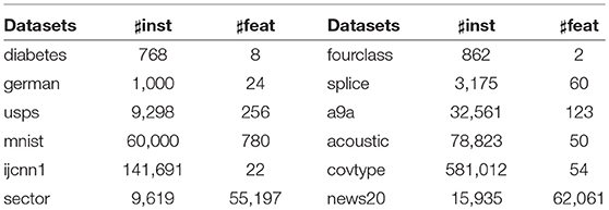
Table 2. Basic information about the benchmark datasets used in the experiments.

For the experiments, the features were normalized by taking $x_i\leftarrow \frac{x_i-\mathrm{\text{mean}}(x_i)}{\Vert x_i\Vert }$ for the large datasets and $x_i\leftarrow \frac{x_i}{\Vert x_i\Vert }$ for the small datasets (diabetes, fourclass, and german). For each dataset, the data is randomly partitioned into 5-folds (4 are for training and 1 is for testing). We generate this partition for each dataset 5 times. This results in 25 runs for each dataset for which we use to calculate the average AUC score and standard deviation. To determine the proper parameter for each dataset, we conduct 5-fold cross validation on the training sets to determine the parameter λ ∈ 10^[−5:1] for SPDAM and for regSOLAM the learning rate ζ ∈ [1:9:100] and the regularization parameter λ ∈ 10^[−5:5] were found by a grid search. The buffer size for OAMseq and OAMgra is 100 as suggested [22]. All experiments for SPDAM and regSOLAM were conducted with MATLAB.

5.3. Evaluation of SPDAM and regSOLAM on Benchmark Datasets

Classification performances on the testing dataset of all methods are given in Table 3. These results show that SPDAM and regSOLAM both achieve similar performances as other state-of-the-art online and offline methods based on AUC maximization. In some cases, SPDAM and regSOLAM perform better than some of the other online learning algorithms. There is a significant improvement in the text classification dataset mnist and covtype. The difference in performance of SPDAM and regSOLAM could be due to the fact since the data is randomly partitioned into two classes, the value of p could be resulting in a higher AUC score.

TABLE 3

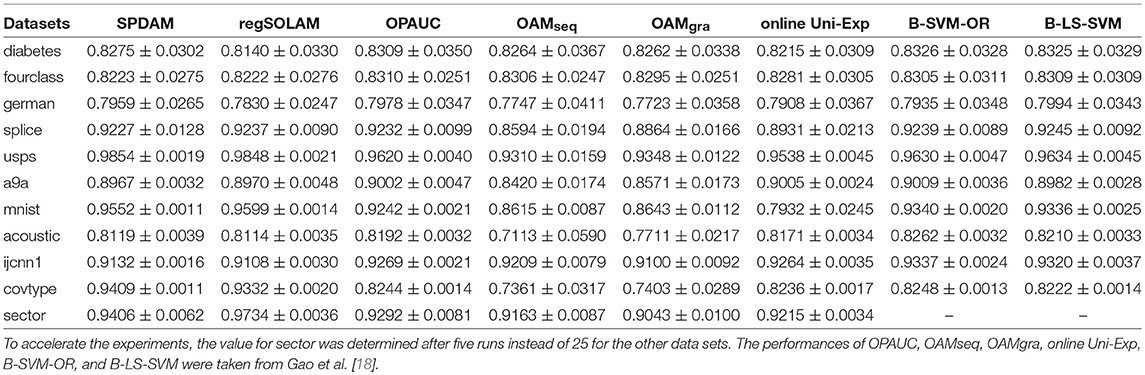
Table 3. Comparison of the testing AUC values (mean±std.) on the evaluated datasets.

However, the main advantage of SPDAM over regSOLAM is the running time performance. SPDAM has a linear convergence rate while regSOLAM has a ${O}(\frac{1}{\sqrt{t}})$ convergence. The theory tells us that SPDAM should be faster than regSOLAM. In Figure 1, we show AUC vs. Iterations for SPDAM against regSOLAM over 3 datasets. The figures show that SPDAM converges faster in comparison to regSOLAM, while maintaining a similar competitive performance as from Table 3.

FIGURE 1

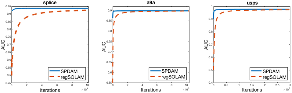
Figure 1. AUC vs. Iteration curves of SPDAM against regSOLAM. For SPDAM, 10% of the data was chosen for a batch size. The optimal value of the parameter λ from SPDAM was used in regSOLAM.

In order to obtain this convergence rate, it is important to pick a large enough batch size (m). As from Theorem 4.1, the value of θ needs to be small for ensuring that SPDAM converges quickly. To ensure a fast convergence, the relationship between σ and θ should be examined. For θ to be small, σ should also be small which can be made possible by increasing the batch size m. If the batch size is too small, SPDAM will result in very poor performance. Figure 2 demonstrates SPDAM on various batch sizes and shows that selecting a larger batch size ensures a faster rate of convergence. A batch size of 10% is sufficient so that SPDAM converges faster than regSOLAM.

FIGURE 2

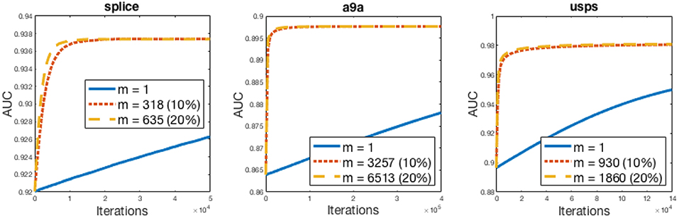
Figure 2. AUC vs. Iteration curves of SPDAM algorithm for various batch sizes. The batch size is a percentage of the number of samples.

6. Conclusion

In this paper, we proposed a stochastic primal-dual algorithm for AUC optimization [18, 22] based upon our previous work that AUC maximization is equivalent to a stochastic saddle point problem. By letting the distribution of ρ as in (7) be uniform, the proposed SPDAM algorithm is shown both theoretically and by experiments that the algorithm achieves a linear convergence rate. This makes SPDAM, given that a large enough batch size is used, faster than regSOLAM. If the batch size is not sufficiently large, SPDAM has poor performance.

There are several research directions for future work. First, the convergence was established using the duality gap associated with the stochastic SPP formulation (7). It would be interesting to establish the strong convergence of the output ${\bar{\text{w}}}_T$ of the regSOLAM algorithm to its optimal solution of the actual AUC optimization problem (3). Secondly, the SPP formulation (3.1) holds for the least square loss. We do not know if the same formulation holds true for other loss functions such as the logistic regression or the hinge loss.

Data Availability

Publicly available datasets were analyzed in this study. This data can be found here: https://archive.ics.uci.edu/ml/index.php.

Author Contributions

All authors listed have made a substantial, direct and intellectual contribution to the work, and approved it for publication.

Funding

This work is supported by NSF grant (#1816227) and was supported by a grant from the Simons Foundation (#422504), and the Presidential Innovation Fund for Research and Scholarship (PIFRS) from SUNY Albany.

Conflict of Interest Statement

The authors declare that the research was conducted in the absence of any commercial or financial relationships that could be construed as a potential conflict of interest.

Acknowledgments

This manuscript is a significant extension of work that first appeared at NIPS 2016 [25].

References

1. Elkan C. The foundations of cost-sensitive learning. In: International Joint Conference on Artificial Intelligence. Vol. 17. Seattle, WA: Lawrence Erlbaum Associates Ltd (2001). p. 973–8.

Google Scholar

2. Metz CE. Basic principles of ROC analysis. In: Freeman LM, Blaufox MD, editors. Seminars in Nuclear Medicine. Vol. 8. Amsterdam: Elsevier (1978). p. 283–98.

PubMed Abstract | Google Scholar

3. Hanley JA, McNeil BJ. The meaning and use of the area under of receiver operating characteristic (roc) curve. Radiology. (1982) 143:29–36. doi: 10.1148/radiology.143.1.7063747

PubMed Abstract | CrossRef Full Text | Google Scholar

4. Fawcett T. ROC graphs: notes and practical considerations for researchers. Mach Learn. (2004) 31:1–38.

Google Scholar

5. Cortes C, Mohri M. AUC optimization vs. error rate minimization. In: Neural Information Processing Systems. Vancouver, BC (2003).

Google Scholar

6. Joachims T. A support vector method for multivariate performance measures. In: International Conference on Machine Learning. Bonn (2005).

Google Scholar

7. Kotlowski W, Dembczynski K, Hüllermeier E. Bipartite ranking through minimization of univariate loss. In: International Conference on Machine Learning. Bellevue, WA (2011).

Google Scholar

8. Rakotomamonjy A. Optimizing area under Roc curve with SVMs. In: 1st International Workshop on ROC Analysis in Artificial Intelligence. Valencia (2004).

Google Scholar

9. Bach FR, Moulines E. Non-asymptotic analysis of stochastic approximation algorithms for machine learning. In: Neural Information Processing Systems. Granada (2011).

Google Scholar

10. Bottou L, LeCun Y. Large scale online learning. In: Neural Information Processing Systems. (2003). Available online at: http://papers.nips.cc/paper/2365-large-scale-online-learning

Google Scholar

11. Cesa-Bianchi N, Conconi A, Gentile C. On the generalization ability of on-line learning algorithms. IEEE Trans Inform Theory. (2004) 50:2050–7. doi: 10.1109/TIT.2004.833339

CrossRef Full Text | Google Scholar

12. Rakhlin A, Shamir O, Sridharan K. Making gradient descent optimal for strongly convex stochastic optimization. In: International Conference on Machine Learning. Edinburgh (2012).

Google Scholar

13. Ying Y, Pontil M. Online gradient descent learning algorithms. Found Comput Math. (2008) 8:561–96. doi: 10.1007/s10208-006-0237-y

CrossRef Full Text | Google Scholar

14. Zinkevich M. Online convex programming and generalized infinitesimal gradient ascent. In: International Conference on Machine Learning. Washington, DC (2003).

Google Scholar

15. Nemirovski A, Juditsky A, Lan G, Shapiro A. Robust stochastic approximation approach to stochastic programming. SIAM J Optim. (2009) 19:1574–609. doi: 10.1137/070704277

CrossRef Full Text | Google Scholar

16. Yu W, Lin Q, Yang T. Doubly stochastic primal-dual coordinate method for regularized empirical risk minimization with factorized data. CoRR. (2015) abs/1508.03390. Available online at: http://arxiv.org/abs/1508.03390

Google Scholar

17. Herschtal A, Raskutti B. Optimising area under the ROC curve using gradient descent. In: Proceedings of the Twenty-First International Conference on Machine Learning. Banff, AB: ACM (2004). p. 49.

Google Scholar

18. Gao W, Jin R, Zhu S, Zhou ZH. One-pass AUC optimization. In: International Conference on Machine Learning. Atlanta, GA (2013).

Google Scholar

19. Kar P, Sriperumbudur BK, Jain P, Karnick H. On the generalization ability of online learning algorithms for pairwise loss functions. In: International Conference on Machine Learning. Atlanta, GA (2013).

Google Scholar

20. Wang Y, Khardon R, Pechyony D, Jones R. Generalization bounds for online learning algorithms with pairwise loss functions. In: COLT. Edinburgh (2012).

Google Scholar

21. Ying Y, Zhou DX. Online pairwise learning algorithms. Neural Comput. (2016) 28:743–77. doi: 10.1162/NECO_a_00817

PubMed Abstract | CrossRef Full Text | Google Scholar

22. Zhao P, Hoi SCH, Jin R, Yang T. Online AUC maximization. In: International Conference on Machine Learning. Bellevue, WA (2011).

Google Scholar

23. Ding Y, Zhao P, Hoi SCH, Ong Y. Adaptive subgradient methods for online AUC maximization. CoRR. (2016) abs/1602.00351. Available online at: http://arxiv.org/abs/1602.00351

Google Scholar

24. Gultekin S, Saha A, Ratnaparkhi A, Paisley J. MBA: mini-batch AUC optimization. CoRR. (2018) abs/1805.11221. Available online at: http://arxiv.org/abs/1805.11221

Google Scholar

25. Ying Y, Wen L, Lyu S. Stochastic online AUC maximization. In: Lee DD, Sugiyama M, Luxburg UV, Guyon I, Garnett R, editors. Advances in Neural Information Processing Systems 29. Curran Associates, Inc. (2016). p. 451–9. Available online at: http://papers.nips.cc/paper/6065-stochastic-online-auc-maximization.pdf

Google Scholar

26. Liu M, Zhang X, Chen Z, Wang X, Yang T. Fast stochastic AUC maximization with O(1/n)-convergence rate. In: Dy J, Krause A, editors. Proceedings of the 35th International Conference on Machine Learning. vol. 80 of Proceedings of Machine Learning Research. Stockholm: PMLR (2018). p. 3189–97. Available online at: http://proceedings.mlr.press/v80/liu18g.html

Google Scholar

27. Rosasco L, Villa S, Vũ BC. Convergence of stochastic proximal gradient algorithm. arXiv:14035074. (2014).

Google Scholar

28. Natole M Jr, Ying Y, Lyu S. Stochastic proximal algorithms for AUC maximization. In: Dy J, Krause A, editors. Proceedings of the 35th International Conference on Machine Learning. vol. 80 of Proceedings of Machine Learning Research. Stockholm: PMLR. (2018). p. 3710–9. Available online at: http://proceedings.mlr.press/v80/natole18a.html

Google Scholar

29. Clemencon S, Lugosi G, Vayatis N. Ranking and empirical minimization of U-statistics. Ann Stat. (2008) 36:844–74. doi: 10.1214/009052607000000910

CrossRef Full Text | Google Scholar

30. Gao W, Zhou ZH. On the consistency of AUC pairwise optimization. In: International Joint Conference on Artificial Intelligence. Buenos Aires (2015).

Google Scholar

31. Zhang Y, Lin X. Stochastic primal-dual coordinate method for regularized empirical risk minimization. In: International Conference on Machine Learning. Lille (2015). p. 353–61.

Google Scholar

32. Joachims T. Training linear SVMs in linear time. In: Proceedings of the Twelfth ACM SIGKDD International Conference on Knowledge Discovery and Data Mining. Philadelphia, PA (2006). p. 217–26.

Google Scholar