1
Theoretical Neurobiology, University of Antwerp, Belgium
2
Computational Neuroscience Unit, Okinawa Institute of Science and Technology, Japan
We describe how the use of the Python language improved the user interface of the program STEPS. STEPS is a simulation platform for modeling and stochastic simulation of coupled reaction-diffusion systems with complex 3-dimensional boundary conditions. Setting up such models is a complicated process that consists of many phases. Initial versions of STEPS relied on a static input format that did not cleanly separate these phases, limiting modelers in how they could control the simulation and becoming increasingly complex as new features and new simulation algorithms were added. We solved all of these problems by tightly integrating STEPS with Python, using SWIG to expose our existing simulation code.
Computational modeling and simulation of signaling pathways has become a valuable and established tool for studying the molecular aspects of biological systems (Bhalla, 2004
; Doi et al., 2005
; Holmes, 2000
; Kuroda et al., 2001
; Lindskog et al., 2006
; Miller et al., 2005
; Smolen et al., 2006
; Stefan et al., 2008
). Modeling such systems consists of identifying the molecular players and describing the stoichiometry and rate constants of their chemical interactions. The resulting system is then often simulated by converting it to a set of coupled ordinary differential equations that can be numerically integrated (Press et al., 2007
).
It has long been acknowledged that the discrete nature of reaction events, caused by the very low numbers of key molecules being present, can make biological reaction systems noisy and affect their behavior on a macroscopic level. This aspect can be brought into the simulation by adding noise terms to the differential equations (Kloeden and Platen, 1999
; van Kampen, 2007
), or more commonly, by simulating the system with Gillespie’s Stochastic Simulation Algorithm or SSA (Gillespie, 1977
) or one of its derivations (Gillespie, 2007
).
For some pathways, however, even more realism is needed. One such case is when the spatial organization and morphology of the cell is known to play an active role in controlling the pathway, e.g. through chemical compartmentalization, spatial gradients and by various transport processes and diffusion (Lemerle et al., 2005
). Such cases are common in neurons because of their complex dendritic arborization (Santamaria et al., 2006
), but of course are not limited to them.
In order to study systems at the level where stochasticity, spatial gradients within complex boundary conditions and diffusion all come into play at the same time, we have developed a simulation platform called STEPS (STochastic Engine for Pathway Simulation) that uses an extension of Gillespie’s SSA to deal with diffusion of molecules in 3-dimensional reconstructions of neuronal morphology and tissue (Wils and De Schutter, 2009
). STEPS computes reactions occurring between diffusing molecules in volumes, and, in addition, also surface reactions to simulate channel fluxes and ligand-receptor binding. Our algorithm differs from a similar approach described in Elf and Ehrenberg (2004)
mainly in that it is based upon the use of tetrahedral meshes which are particularly well-suited for representing biological morphology and that we avoid the use of a heap structure.
In this paper, based on a presentation made at the FACETS CodeJam #2 workshop ‘Building the meta-simulator tool-chain: leveraging Python for a robust and efficient workflow in computational neuroscience’, describes how Python scripting is used for working with models in STEPS. We also show how, in this particular problem domain, adding Python scripting improved the quality and maintainability of STEPS in a fundamental way.
Brief Description of Steps Algorithm
Stochastic simulation of reaction-diffusion processes can occur in a number of ways. One way is to track each reacting molecule as an independent particle that undergoes Brownian motion and occasionally collides with one of the other tracked molecules. This is the approach taken by such programs as M-Cell (Stiles and Bartol, 2001
) and Smoldyn (Andrews and Bray, 2004
).
Another approach is voxel-based; here one keeps track of how much molecules are present from any given species within a set of small volumes. By keeping these reaction volumes or voxels small enough, we can state that the concentration gradients within each voxel are negligible: the voxel is approximately well-mixed. Then we can apply SSA (Gillespie, 1976
) by adding an extra reaction rule for each type of molecule for its diffusion step from one voxel to a neighboring one. Thus SSA handles both diffusion processes and reaction mechanisms from within one single simulation framework. Though this approach is abstracted more from the underlying physical mechanisms than modeling Brownian motion, it offers a number of advantages. Because diffusion is uncoupled from chemical reaction, the modeler can decide for each type of molecule, considering the timeframe being simulated, whether it makes sense to implement diffusion or not. At the coding level, much less bookkeeping is necessary because one does not track individual molecules, giving rise to leaner and potentially faster code. It also facilitates combining SSA with approximate, faster methods such as tau-leaping (Gillespie, 2001
).
STEPS simulates molecular reaction-diffusion in volumes which are bounded by membranes. These membranes can contain stationary reacting molecules, including channel proteins. To simulate the behavior of these systems, STEPS adapts the Direct Reaction Method version of SSA (Gillespie, 1976
) for large systems by storing the propensity values for each process in a search tree. STEPS 0.4 implements two distinct stochastic solvers: a spatial solver (called tetexact) and an auxiliary well-mixed solver (called wmdirect, this does not model diffusion). Such well-mixed solvers are useful assistants because setting up a spatial model can benefit greatly from analyzing and tuning parts of the biochemical model under simpler conditions (Wils and De Schutter, 2009
). In the future additional solvers will be added, including a deterministic one (based on Runge-Kutta integration; Press et al., 2007
) and an extension of tetexact that includes diffusion in membranes.
Steps Workflow
Figure 1
shows a typical workflow for developing and simulating a 3-dimensional reaction-diffusion system and how the different phases can relate to each other. The first step, biochemical modeling, consists of describing reaction stoichiometry and selecting reaction rates and diffusion constants. Since this is independent to a large degree of the actual algorithm that will be used for simulation (i.e. numerical integration of ODE’s vs stochastic simulation; with or without diffusion; …), it is common practice to import and compose this type of information from previous modeling efforts through formats such as SBML (Hucka et al., 2003
)
1
.
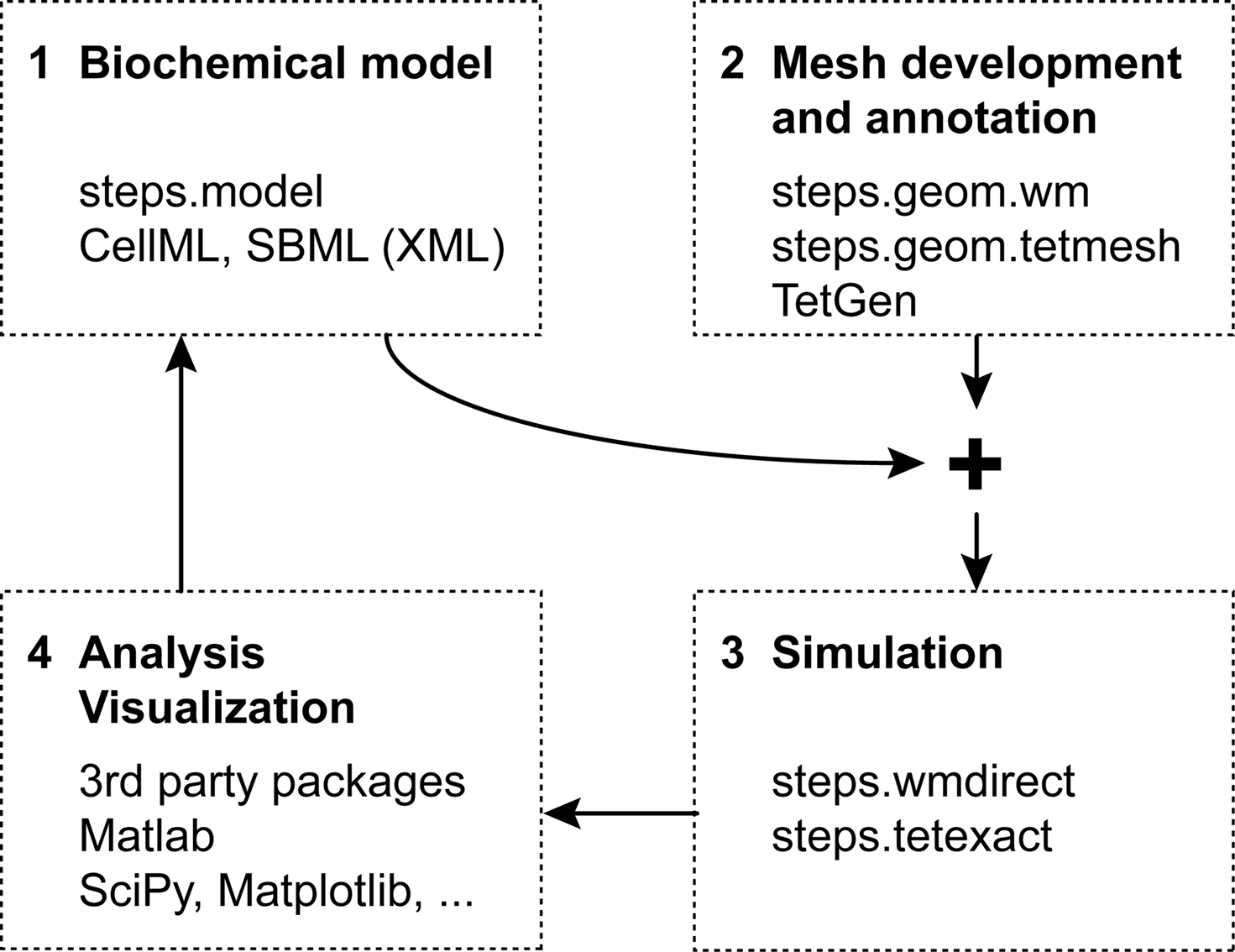
Figure 1. Workflow for reaction-diffusion modeling with four phases.
Mesh generation, or more generally speaking describing the geometric boundaries of the problem, is another step. Since tetrahedral meshes are supported both by stochastic solvers (Wils and De Schutter, 2009
) as well as more traditional methods based on numerical integration of systems of partial differential equations (Ferziger and Peric, 2002
), they are fairly independent of the algorithm that will be used at a later stage. In addition, a mesh can be reused with multiple modeling and simulation studies, a distinct advantage considering that their generation can be a rather elaborate task, especially for meshes based on imaging data (Means et al., 2006
).
Because of their independence, the previous two phases can easily be performed in parallel, or even by separate groups. The only point where everything needs to come together and link up, is at the start of the third phase: running a simulation. This phase is the focus of STEPS and will be detailed below.
The fourth and final phase is the most important and daunting of all: collecting the simulation results, analyzing them and, if necessary, readjusting the biochemical model. Even more than was the case with the first two phases, different modelers will want to rely on different tools for this task. A logical option for STEPS modeling results are the many packages already available for Python (Scipy, Matplotlib, …).
In the rest of this section, we will implement the simple toy model in Figure 2
to examine in more detail how different STEPS packages support each of the first three phases of our modeling cycle independently. We will show how easy it is to go from well-mixed to spatial simulations and back. We will then conclude our discussion of STEPS by looking at it from an architectural point of view and discuss the multiple roles that Python plays in allowing STEPS users to combine all the components of this cycle into a modeling pipeline.
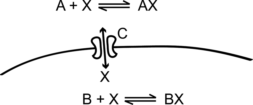
Figure 2. This simple model, which is inspired by calcium dynamics, will be used to explain the STEPS implementation. It consists of two distinct chemical environments separated by a membrane. A substance X can be bound to buffer molecules of type A and B or it can be transported through a membrane channel C from one volume to the other.
Biochemical Model Description
The objects that together define the biochemical aspects of a STEPS model are written directly in Python and are grouped in package steps.model. The following snippet of Python code shows how to implement the simple toy model from Figure 2
using these objects:
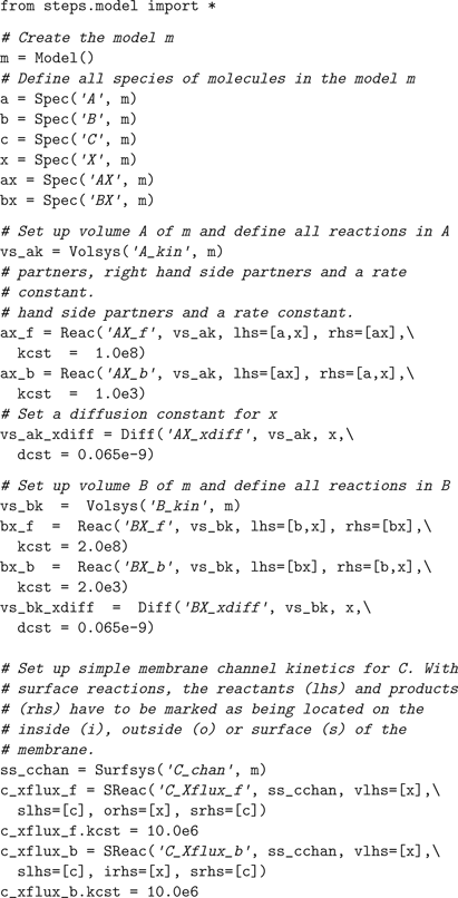
As one can see the model is created through a series of Python function calls that map onto STEPS code (see Figure 4
). Volume systems (objects of class Volsys) describe the chemical properties of volume solutions, which comprise the stoichiometry and rate constants of reaction channels and the diffusion constants for all diffusing species in that solution. Surface systems (objects of class Surfsys) describe the chemical properties of membranes, such as ligand-receptor binding and unbinding or channel currents. Note that some information is given implicitly: because no diffusion constants are supplied for the molecular species A, B and AX, BX these are considered immobile.
Demonstrating the independence between the model construction phases mentioned earlier, this code shows that this level of description is completely separate from the geometry or the spatial ‘location’ of these volume and surface systems, and of the initial and boundary conditions or simulation events. Volsys and Surfsys are essentially just static template objects that group together related reaction rules and that will, at a later point in time, be instantiated on the actual simulation geometry. This uncoupling, which is somewhat different from the approach used in SBML where the kinetic equations are usually mixed with compartment definitions and initial conditions, makes it easy for modelers to compose and recombine their biochemical models with different geometric descriptions. Since the objects themselves are in the end still just static hierarchies, a linking point with formats such as SBML or CellML
2
remains.
3D Boundaries: Tetrahedral Meshes
STEPS uses unstructured, tetrahedral meshes (Ferziger and Peric, 2002
; see Figure 3
A for an example) to describe the geometric domain in 3-dimensional detail. In these meshes, elements are not numbered along principal axes and do not have to be perfectly regular, allowing them to adapt to the local level of detail and to follow an arbitrary set of domain boundaries rather smoothly. We will not describe the Python scripting (steps.mesh) in detail, but instead focus on the conceptual approach.
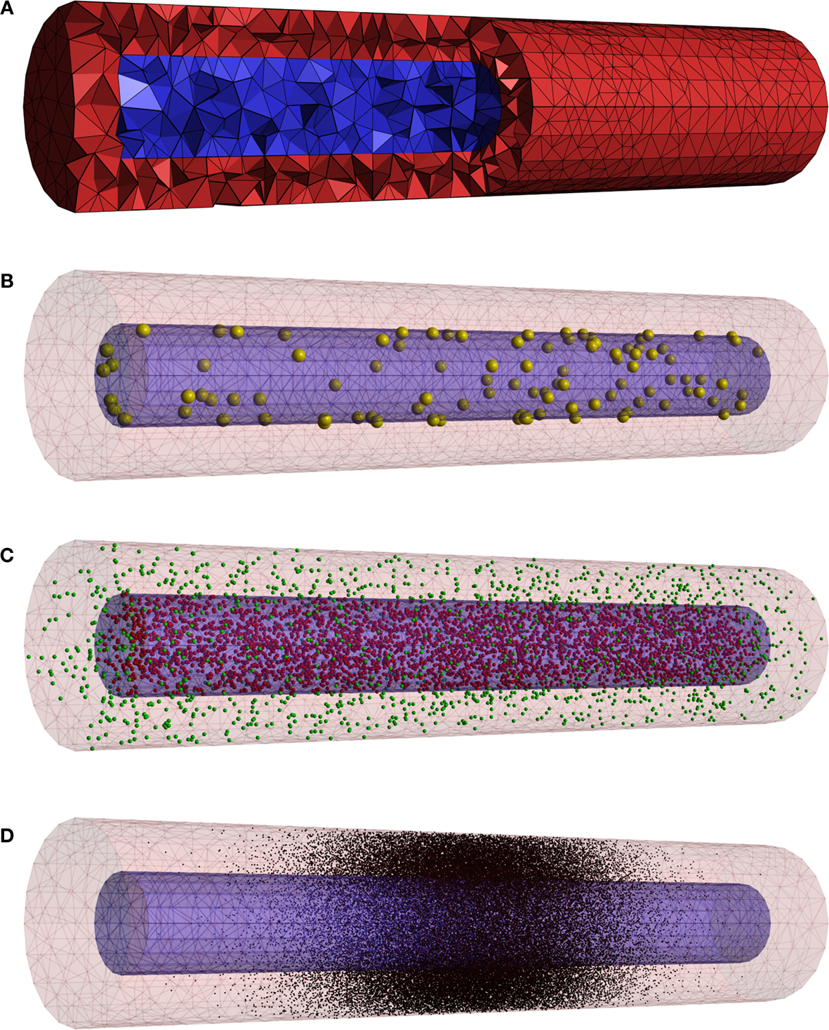
Figure 3. The mesh used in the code examples for setting up initial conditions. (A) This opaque view with a cut-out shows that 21090 tetrahedons are used to describe one cylinder surrounding another one. (B) Membrane channels C are distributed randomly over the inner membrane. (C) A uniform initial distribution for molecules A and B. (D) A Gaussian distribution in the center of the outer cylinder for X.
To organize the simulation space into biological structures STEPS uses the notion of ‘compartment’ for volumes and ‘patches’ for surfaces. For example, compartments can represent physical regions such as the cytoplasm, ER lumen or cellular exterior. In order to be useful for a simulation, the tetrahedral mesh has to be annotated so that each tetrahedron is assigned to a ‘compartment’ (objects of class Comp) and each triangle is assigned to a ‘patch’ (objects of class Patch). When these objects are used directly, instead of a mesh, it is possible to describe a well-mixed geometry that can be used in well-mixed simulations, similar to the compartments found in SBML.
Eventually, Comp and Patch objects will refer to one or more volume systems or surface systems, respectively. As detailed in the next section, these references are resolved during the initialization phase of a simulation, when a model description is combined with a mesh object. At any point prior to simulation, however, these references are stored simply as string values, allowing users to manipulate meshes independently of any biochemical model. A mesh can be stored with or without such references, making it easy to reuse a mesh for simulating many different biochemical models.
As is the case with the objects of package steps.model, meshes are Python objects that can be manipulated using Python scripts or from the Python command line. It therefore becomes easier to automate many tasks and to write custom importers or exporters for various forms of 3D data. Currently, STEPS directly supports importing meshes from the freely available tetmesh generator TetGen
3
.
In the following snippet of code, we load a previously generated mesh (Figure 3
A) stored in an archive. The mesh, which is used for demonstration purposes only, consists of two cylindrical compartments (called outer and inner) separated by a membrane patch called imem. This could represent, for example, a segment of dendrite with endoplasmic reticulum in its center. We link the mesh to our toy model by assigning these compartments and patches to volume systems and surface systems as needed.
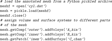
Notice that we only needed three line of code to perform this link to a fairly complex mesh.
Running a Simulation
The third phase in the modeling cycling is to simulate the model with a numerical solver. To do this in STEPS, a solver object must be created. This basically consists of one line of code in which this object is created and initialized with the biochemical model, a geometric description and a random number generator. It is from within the constructor of this solver object that all references from the Comp and Patch objects to the Volsys and Surfsys objects are resolved in order to create the appropriate data structures needed to represent the state of the simulation.
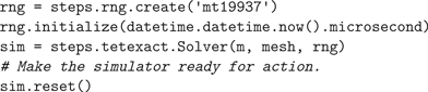
The spatial solver (steps.tetexact) used in this example only accepts tetrahedral meshes, whereas the well-mixed solver (steps.wmdirect) can accept both a well-mixed description or a tetmesh, from which the well-mixed features can be transparently extracted. Note that in the latter case the definition of diffusion constants in our toy model would be ignored automatically. The only change needed for setting up a well-mixed simulation would be in the third line of the code example, where steps.wmdirect.Solver would be evoked instead.
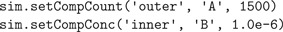
All current and future solver objects, regardless of their underlying algorithm or of their spatial or well-mixed nature, provide the same API through which the modeler can access the internal state of the simulation from within Python, in order to set initial conditions and to control the simulation. This internal state includes the local amount of molecules for different species, but also whether these species are buffered, the reaction and diffusion constants and whether reaction channels are active or not. All of these properties can be manipulated for individual tetrahedrons and triangles (in mesh-based solvers), or for entire compartments and patches at a time (in both mesh-based and well-mixed solvers). In Figures 3
B–D we show three possible initial conditions for the concentration of X from our toy model. We first inject 100 channels of species C in the inner membrane imem (Figure 3
B):

Next, we inject 1500 molecules of species A in the outer compartment and set the concentration of species B in the inner compartment to 1 μM, spread out uniformly (Figure 3
C):
Note that in both examples the position of channels or molecules is automatically randomized with uniform distributions. Because the API also allows access to the simulation state at the level of individual tetrahedrons, we can program arbitrarily complex initial conditions and runtime events. In the next piece of code we show how this can be used to generate a normally distributed pulse injection of X in the outer compartment with a given peak amplitude and width centered in the middle (Figure 3
D):
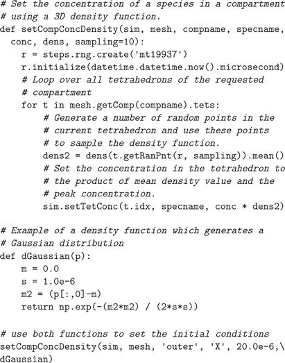
These examples show the great flexibility that Python offers in setting up initial conditions for the simulation. In addition, the API also features the actual control functions that allow one to reset a simulation, to advance the simulation to some future time and to sample the simulation state.
Why Python?
To understand the design of the STEPS software package, a short history is useful. An earlier incarnation of STEPS consisted of a single standalone C++ application. Being focused on the simulation algorithm itself, not much thought was given to issues related to model description and simulation control and these aspects were put together in a single custom XML-based format. We didn’t use SBML at the time because it lacked support for models with detailed 3D features. Meshes had to be stored in a separate custom data format and were referenced by filename from within these XML input files.
The limitations of our first implementation became apparent rather quickly. We discovered that, because of the spatial aspects, describing the initial state of a 3D reaction-diffusion system is more complicated than describing the initial state of a well-mixed simulation. People might not just want to set initial values in compartments as a whole, but inject molecules or manipulate rate constants using more sophisticated geometric patterns, for instance using a Gaussian distribution to mimic the result of a laser uncaging event (Wang and Augustine, 1995
; see Figure 3
D). Sometimes the simulation might require this release pattern to be confined to a particular compartment; other simulations might want the pattern to be applied globally.
Coming up with an XML-based way of describing a wide range of in-simulation events, a problem similar and closely related to the problem of setting up initial conditions, and output generation proved to be quite difficult. By far the most common use case would be to have events occur on specific times during the course of a simulation. But what if an event would have to depend on some condition being met, such as the concentration of some species reaching a threshold? We ended up with an increasingly rich fauna of trigger, action and output objects which covered many possibilities, but which was complicated and costly to maintain and in the end still left many rare but sensible use cases uncovered.
When at some point we also started thinking about supporting well-mixed solvers directly from within STEPS, we decided that our old approach had reached its limits and set out to redesign STEPS by integrating it closely with a fully-featured scripting language. Python was chosen because it is a mature language, simple to learn and already had a widespread user base in the computational sciences, with a wide selection of third-party packages and documentation to match. As described above, its object oriented features allowed us to express the relationship between well-mixed and spatial models in a way that facilitates switching between the corresponding classes of simulators. Python’s excellent XML features will allow us to keep up with projects such as SBML when their support for spatial modeling matures. Finally, Python can be used to integrate many miscellaneous tasks related to simulation that would otherwise typically be done with shell scripting. Examples are copying files to their right location, cleaning up, initiating a data processing or compacting method directly after a simulation finishes, etc.
The redesign was a major effort. The only part that could be reused from the old STEPS was the core simulator code, i.e. the solver currently known as tetexact. Everything else had to be rewritten following the modeling workflow described in Figure 1
. We designed the solver API mentioned above and implemented it for our two current solvers. These API implementations were then exposed to Python using SWIG
4
, where they were further wrapped in a Python-side Solver base class that performs argument checking and provides some extra higher-level functionality. Much of the code for setting up a solver is the same for all current and future solvers and was therefore put in a shared set of C++ files. This reduces the amount of ‘plumbing code’ that needs to be written for a new solver, while still allowing considerable freedom in choosing the ultimate algorithm-specific internal data structures.
The main flaw of our first version of Pythonizing STEPS, as shown in Figure 4
, is the many layers that have to be passed to go from calling a solver object method to the actual solver code and back. This may become a performance bottleneck when one is running a simulation that is interrupted repeatedly over small time intervals. This problem may be resolved in several ways. We can recode the Python-side Solver class, which is shared by all solvers, in C++ and derive an actual individual solver by overriding protected virtual methods. To avoid even the cost of virtual calls in this scenario, we can employ the Curiously Recurring Template Pattern (Vandevoorde and Josuttis, 2003
). Alternatively, we can switch from SWIG to Boost.Python
5
, an ingenious method of exposing C++ code to Python that does not result in a Python-side shadow class, as is the case with SWIG.
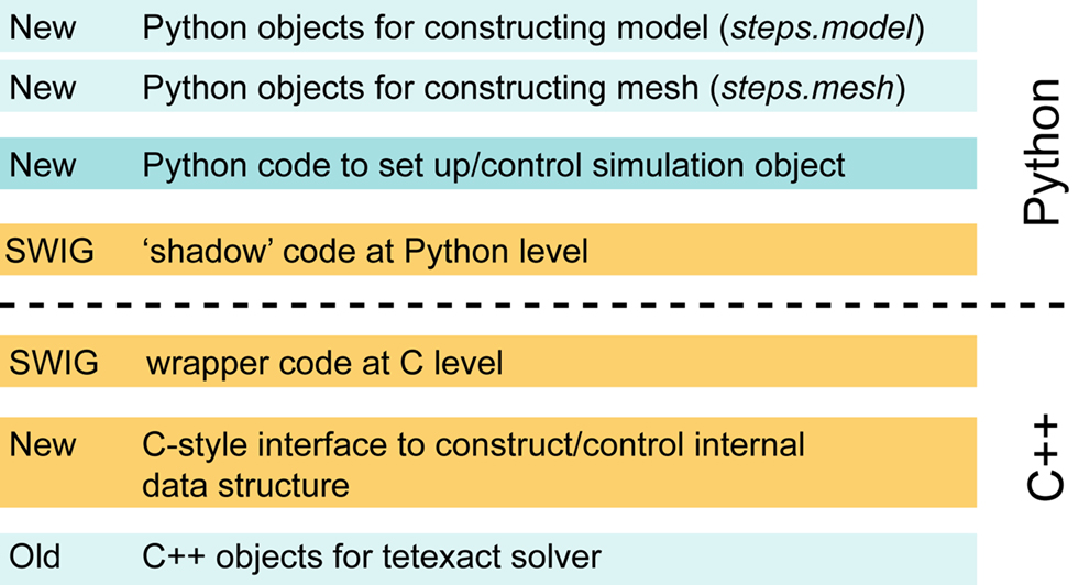
Figure 4. Layered view of STEPS code after exposing it to Python with SWIG.
We have described how STEPS mixes C++ with Python scripting to give modelers greater freedom in setting up and simulating a model, while maintaining the efficiency of compiled and optimized C++ code. We described how going the extra mile to make a scientific simulator fully scriptable in this way has considerable advantages. Because of the many scientific computing packages already available for Python, computational scientists are encouraged to develop sophisticated pipelines in which modeling, simulation and even post processing and visualization are highly automated. In addition, we find that the neural simulators such as Neuron (Carnevale and Hines, 2006
) and Moose
6
have committed to supporting Python, leading some to forward the challenging but intriguing possibility of using Python to actually ‘glue’ together simulations (Cannon et al., 2007
). One should keep in mind, however, that naively using an interpreted language like Python to exchange and map state information between simulators at each time step might quickly run into performance and numerical issues that could be avoided only by deeper integration at the algorithmic level. Alternatives like the MUSIC project (Ekeberg and Djurfeldt, 2008
) might therefore be better suited for this.
Like many before us, we have successfully used SWIG to expose our existing C++ simulation core to Python. The main technical issue that we encountered is the many layers between the user script and the C++ code which, as mentioned, can be resolved by porting the solver interface to C++ and possibly by switching to Boost.Python.
In the specific context of modeling 3D reaction-diffusion simulations we found that using Python had a large advantage for describing a complex internal state. There are many ways in which a biologist might want to set up and control this state and sample it for output. Switching to a scripting language allowed us to eliminate a great deal of complexity that was ultimately caused by sticking to a static, purely declarative input format in which model and simulation were thoughtlessly mixed. Since maintaining a backwards compatible API of basic getter/setter functions is less of an effort than designing and maintaining an increasingly ‘baroque’ set of trigger, action and output objects, we expect that this investment will keep paying off as STEPS keeps growing by adding more solvers and more capabilities. In other words, our switch to Python has actually saved us quite some time.
Finally, we believe that our experience suggests that a language like Python, as was proposed earlier in Cannon et al. (2007)
, can play a positive role in supporting the development of formal standards for sharing scientific models. Mirroring the requirements of understanding biology itself, biological simulators will necessarily become more complex and will be able to simulate more and more aspects of the living cell. Codes such as M-Cell (Stiles and Bartol, 2001
), MesoRD (Hattne et al., 2005
), Smoldyn (Andrews and Bray, 2004
) and also STEPS expand on the idea of ODE-based, well-mixed simulations of reaction kinetics by adding stochasticity and spatial processes such as diffusion. But this is only the beginning. The future will see developments such as simulations of electrophysiological phenomena in high 3D detail or full electrodiffusion (Lopreore et al., 2008
), volume-occupying molecules (Gillespie et al., 2007
; Schnell and Turner, 2004
), dynamic meshes whose shape is controlled by simulated chemistry and, as mentioned earlier, possibly even the integration of simulators that work on different scales.
The designers of formal standards, such as SBML, can not be expected to keep up with these new trends as they come out, and still maintain a clean standard. This fact flows from a fundamental tension between on the one hand having a clean, simulator-independent standard for publishing models, and on the other hand the turbulent, seemingly endless expansion of exactly what is required in a biological model to be relevant and how to breathe it all to life on a computer. The advantages of having such standards is obviously too great to discard (Bergmann and Sauro, 2008
), and successes have been achieved to where classes of modeling efforts have sufficiently crystallized, together with the methods to simulate them (Hucka et al., 2003
). The combination of Python and XML eases this tension by allowing projects that explore new types of simulations to mature independently from the standards for model sharing. It allows them to catch up with each other whenever and wherever it makes sense to do so.
The authors declare that the research was conducted in the absence of any commercial or financial relationships that could be construed as a potential conflict or interest.
This work was supported by grants from GOA (UA, Belgium), HFSP and OIST (Japan).
Our software is released under the GNU public license and can be downloaded from http://sourceforge.net/projects/steps
.
Ekeberg, Ö., and Djurfeldt, M. (2008). MUSIC – Multisimulation Coordinator: Request For Comments. Nature Precedings. Available at: http://dx.doi.org/10.1038/npre.2008.1830.1
.
Hucka, M., Finney, A., Sauro, H. M., Bolouri, H., Doyle, J. C., Kitano, H., Arkin, A. P., Bornstein, B. J., Bray, D., Cornish-Bowden, A., Cuellar, A. A., Dronov, S., Gilles, E. D., Ginkel, M., Gor, V., Gorvanin, I. I., Hedley, W. J., Hodgman, T. C., Hofmeyr, J. H., Hunter, P. J., Juty, N. S., Kasberger, J. L., Kremling, A., Kummer, U., Le Novère, N., Loew, L. M., Lucio, D., Mendes, P., Minch, E., Mjolness, E. D., Nakayama, Y., Nelson, M. R., Nielsen, P. F., Sakurada, T., Schaff, J. C., Shapiro, B. E., Shimizu, T. S., Spence, H. D., Stelling, J., Takahashi, K., Tomita, M., Wagner, J., and Wang, J. (2003). The systems biology markup language (SBML): a medium for representation and exchange of biochemical network models. Bioinformatics 19, 524–531.