1
Bernstein Center for Computational Neuroscience, Freiburg, Germany
2
Computational Neuroscience, Faculty of Biology, Albert-Ludwig University, Freiburg, Germany
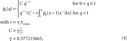
3
Honda Research Institute Europe, Offenbach, Germany
4
Theoretical Neuroscience Group, RIKEN Brain Science Institute, Wako City, Japan
5
Brain and Neural Systems Team, Computational Science Research Program, RIKEN, Wako City, Japan
Hebbian learning in cortical networks during development and adulthood relies on the presence of a mechanism to detect correlation between the presynaptic and the postsynaptic spiking activity. Recently, the calcium concentration in spines was experimentally shown to be a correlation sensitive signal with the necessary properties: it is confined to the spine volume, it depends on the relative timing of pre- and postsynaptic action potentials, and it is independent of the spine's location along the dendrite. NMDA receptors are a candidate mediator for the correlation dependent calcium signal. Here, we present a quantitative model of correlation detection in synapses based on the calcium influx through NMDA receptors under realistic conditions of irregular pre- and postsynaptic spiking activity with pairwise correlation. Our analytical framework captures the interaction of the learning rule and the correlation dynamics of the neurons. We find that a simple thresholding mechanism can act as a sensitive and reliable correlation detector at physiological firing rates. Furthermore, the mechanism is sensitive to correlation among afferent synapses by cooperation and competition. In our model this mechanism controls synapse formation and elimination. We explain how synapse elimination leads to firing rate homeostasis and show that the connectivity structure is shaped by the correlations between neighboring inputs.
The connectivity structure of the cortex was found to be surprisingly dynamic in vitro and in vivo (Bonhoeffer and Yuste, 2002
). Synapse formation and elimination exhibit a marked dependence on spiking activity, where higher activity promotes synapse formation (Le Be and Markram, 2006
). Based on geometric considerations, Stepanyants et al. (2002)
, Chklovskii et al. (2004) and Stepanyants et al. (2007)
suggest as a basic design principle of the cortex the potential of any pair of neurons to form a connection on small length scales of a few hundred micrometers together with an activity dependent selection mechanism. This idea is supported by direct observation of spines approaching presynaptic partners in a promiscuous manner (Kalisman et al., 2005
). Of these structurally possible (potential) synapses, only a small fraction (0.12–0.34) is actually realized (Stepanyants et al., 2002
), and transitions from potential to actual synapses are observed in vitro at rates of up to 1.2 per cent per hour during increased spiking activity (Le Be and Markram, 2006
). These newly formed, immature synapses are weaker than mature ones. Synapse pruning mostly affects weak, but already mature synapses. The relation of synaptic strength to synapse formation and synaptic death indicates that long term potentiation (LTP) and synapse formation may be controlled by similar mechanisms and the same may hold for long term depression (LTD) and synapse pruning. The observation of increased connectivity after prolonged spiking activity also prompts for a synapse pruning mechanism, which restores the typical synapse density. In support of this hypothesis, not only in the developing cortex, but also in adult monkeys in vivo, synaptic boutons emerge and disappear with rates of 7 per cent per week (Stettler et al., 2006
).
The functional role of synapse formation and elimination is not well understood, but theoretical studies have exposed the benefits of the capability of structural remodeling (Chklovskii et al., 2004
; Stepanyants et al., 2002
). Due to the fact that the number of potential presynaptic partners of a neuron easily exceeds the actual number at any point in time by an order of magnitude, each synapse carries three to four bits of structural information. In the framework of spiking associative memories this beneficial functional role of structural plasticity can be exploited to increase the memory capacity (Knoblauch, 2006
; Knoblauch et al., 2007
). Therefore, synaptic formation and elimination is a candidate process for long term information storage in cortical networks during development and adulthood alike.
The microscopic mechanisms leading to the formation of new synapses and to the elimination of existing ones have not yet been completely revealed. However, there is some evidence, that newly formed synapses are created in an intermediate, silent state (Cohen-Cory, 2002
; Kalisman et al., 2005
). These frequently encountered silent synapses lack AMPA receptors but have NMDA receptors (Atwood and Wojtowicz, 2004
). They bear a high potential for remodeling the neural circuit, since they can easily be converted into active synapses. The most probable mechanism is the translocation of AMPA receptors into the postsynaptic density (PSD). This is also observed (Cohen-Cory, 2002
; Shi et al., 1999
) during LTP for which NMDA receptor activation is a necessary precondition.
There is strong indication that synapse formation and synapse pruning are controlled in a similar way as LTP and LTD (Lüscher et al., 2000
). Furthermore, Le Be and Markram (2006)
found that the same antagonists prevent LTP and synapse formation, and conclude that the underlying mechanisms may be similar. Calcium entering the postsynaptic site through NMDA receptors is a probable messenger causing synapse maturation (Atwood and Wojtowicz, 2004
). For the induction of LTP and LTD, which in parts come about by modulating the number of postsynaptic AMPA receptors, Cormier et al. (2001)
showed that both depend in a threshold like fashion on the intracellular calcium peak amplitude: higher amplitudes lead to LTP and lower ones to LTD.
Spike pairing experiments showed the calcium signal in spines to depend on the correlated activation of the pre- and postsynaptic site: Nevian and Sakmann (2004
, 2006
) found a marked dependency on the relative timing and independence on the position of the spine along the dendrite, making the NMDA receptor mediated calcium level in a spine an attractive candidate substrate to convey information about the correlation between presynaptic and postsynaptic activity.
For the calcium signal in a spine to control synaptic maturation or synaptic death it must activate a downstream signaling cascade. Calcium/calmodulin dependent kinase II (CaMKII) is a calcium activated kinase, which is crucial for the LTP of a synapse. In its activated state it can phosphorylate several structures among them AMPA receptors which respond with increased conductivity. There is also evidence, that CaMKII is involved in the insertion process of new AMPA receptors into the PSD. This causes LTP or turns a silent synapse (only having NMDA receptors) into an active one having AMPA and NMDA receptors. There is recent evidence from detailed biophysical modeling studies (Graupner and Brunel, 2007
) that the activity dependent calcium influx can activate CaMKII in a bistable fashion and hereby explain spike timing dependent synaptic plasticity (STDP). For a recent review of phenomenological models of STDP see Morrison et al. (2008)
.
CaMKII forms holoenzymes of two ring molecules consisting of six subunits each. A subunit can either be active or inactive. Transitions between the inactive and the active state are triggered by calcium signals of different amplitudes. Short and weak calcium signals typically lead to activation of a single subunit by binding calcium or calmodulin to it. After the calcium level has dropped, unbinding of calcium and hence deactivation occurs within 0.1–0.2 s. At larger calcium concentrations an active subunit of the molecule (to which calcium is already bound) can phosphorylate the neighboring subunit. This only requires one additional calcium molecule to bind to the second subunit to expose its phosphorylation site. So phosphorylation can propagate along the ring and the molecule remains active even after calcium has returned to the resting level. At resting calcium concentrations, protein phosphatase 1 (PP1) can dephosphorylate an active subunit, but a neighboring active site can immediately rephosphorylate it again. This regenerating effect explains the long time scales of several minutes for the deactivation of groups of active CaMKII molecules. Even longer time scales of hours of persistent activity are found at resting calcium concentrations in the special chemical environment of the PSD, where the concentration of PP1 is low compared to the number of CaMKII subunits. For a comprehensive review see Lisman et al. (2002)
. Detailed biophysical simulations (Miller et al., 2005
) have confirmed bistability between an active and an inactive state of whole populations of approximately 20 holoenzymes. This effect is due to saturation of the phosphatase in the active state. The study found life times of both states in the range of 100 years. The time scale of the attractor dynamics is on the order of tens of minutes, but for strong fluctuations of the calcium signal the bistability vanishes. Calcium can not only activate CaMKII (either directly or via calmodulin), but also protein phosphatases like calcineurin and protein phosphatase 1, which dephosphorylate CaMKII. These phosphatases have a higher affinity to calcium than CaMKII. Therefore, they become active at lower calcium concentrations and counteract the phosphorylation of CaMKII. This is in agreement with the finding that LTD in CA1 dendrites can be induced if the calcium concentration is below 180 nM, while LTP requires it to exceed 540 nM (Cormier et al., 2001
). For a review see Cavazzini et al. (2005)
.
To our knowledge, previous models for structural plasticity either used simplified neuron models (Butz et al., 2008
; Dammasch et al., 1986
) or plasticity rules depending on the firing rate alone and not taking into account formation and death of individual synapses (van Ooyen et al., 1995
). Consequently correlation dependent structure formation is outside the scope of these works. In this modeling study, we investigate how the biologically known pathways outlined above interplay to achieve a mechanism capable of detecting correlation between the presynaptic and the postsynaptic spiking activity. We focus on the calcium control hypothesis: the calcium signal mediated by NMDA receptors is the beginning of the signaling cascade. The main features of NMDA receptors entering our model are: (1) Their fast binding to glutamate followed by slow unbinding. (2) The quasi-instantaneous removal of the magnesium block upon postsynaptic depolarization to open the channel. In these assumptions, our model is similar to previous work by Shouval et al. (2002) on a mathematical model to explain spike timing dependent plasticity (STDP) based on the properties of NMDA receptors and the calcium control hypothesis. In contrast to their work, we assume the postsynaptic depolarization by the backpropagating action potential (bpAP) to be a short event.
The next stage of the signaling pathway in our model is a calcium controlled bistable effector molecule, like e.g. CaMKII. The important properties for our model are: (1) The long time constants of sustained activation of each individual molecule by high calcium concentrations (bistability). We are interested in the regime, where calcium fluctuations dominate the activation dynamics and the slower attractor dynamics causing bistability of the whole population of molecules is negligible. (2) The ability of the kinase to influence synaptic plasticity via AMPA receptor insertion. We assume a minimum amount of the kinase to be necessary for promoting synapses from silent to functional and we assume that there a minimal amount of active kinase is required to prevent synapse death. (3) Two disjoint ranges of calcium concentration that control the transitions between the inactive and the active state of each molecule. (4) The relatively low number of molecules, which makes a statistical description essential. We derive a model for correlation detection based on this pathway and investigate its dynamics under realistic conditions of irregular spike trains. We show that the model represents a viable mechanism to sense correlation between the pre- and postsynaptic activity. Controlling synaptic pruning, it can implement a firing rate homeostasis. Cohen-Cory (2002)
already suspected, that activity-dependent remodeling selectively stabilizes coactive incoming synapses and destabilizes others. We demonstrate that such cooperation and competition between synapses naturally emerges from the microscopic model and that a neuron can learn the correlations between neighboring inputs.
In the section “Spike Time Dependence of Postsynaptic Calcium Concentration” we explain the origin of spike timing dependence of the postsynaptic calcium concentration, mention the main findings of recent imaging experiments, and develop a model for the peak amplitude of the postsynaptic calcium signal. We show it to qualitatively reproduce the experimental findings. In the section “Ca2+ Transients Caused by Correlated Irregular Spiking” we show that for irregular spiking activity this model predicts a distinct dependency of the observed postsynaptic calcium signal on the correlation between the presynaptic and the postsynaptic spiking events. The section titled “A Counter for Correlated Events” derives a biologically motivated model of a mechanism to “count” correlated events and therefore to assess the degree of correlation between the presynaptic and the postsynaptic activity. The section titled “Rate Homeostasis by Synaptic Pruning” shows that controlling synaptic pruning by this correlation measure can act as a rate regulation for the postsynaptic neuron at low rates. In the section “Cooperation and Competition by Spatial Input Correlation” we demonstrate that cooperation and competition between synapses depends on the correlation between neighboring inputs and that a synaptic pruning process manifests these input correlations in the resulting network structure. The last section discusses our results.
All simulations were carried out with the NEST simulation software (Gewaltig and Diesmann, 2007
) using the computationally efficient implementation of synaptic maturation and death provided in the section “Algorithmic Implementation of Synapse Maturation and Synapse Death” in Appendix. Preliminary results have been presented in abstract form (Helias et al., 2007
).
Spike Time Dependence of Postsynaptic Calcium Concentration
In this section we show, that the calcium peak amplitude in a spine in good approximation depends exponentially on the temporal difference of the presynaptic and the postsynaptic spiking and that the calcium influx is largest, if the presynaptic cell fires shortly before the postsynaptic cell. This makes the calcium signal an appropriate candidate carrier of information on causal correlation.
Figure 1
A illustrates the situation at a synapse subject to a spike pairing protocol. The principal mechanism causing the dependence of the postsynaptic calcium signal can readily be understood. With each presynaptic spike a small amount of glutamate is released, increasing the glutamate concentration ρglu at time tglu. Glutamate binds to a fraction of the postsynaptic NMDA receptors. There is experimental evidence (Mainen et al., 1999
) that only a fraction n(t) of the NMDA receptors bind to glutamate. n(t) reaches its maximum n0 after a rise time of τrise,nmda  5 − 10 ms. We choose this maximum obtained for a single presynaptic release to be the unit of n. After the glutamate concentration ρglu(t) has decayed back to its resting value, the receptors unbind and n(t) decays back to 0. As long as the postsynaptic spine is not depolarized, the NMDA receptors are blocked by magnesium and thus have a low conductance (Jahr and Stevens, 1990a
,b
). Arrival of a postsynaptic back-propagating action potential (called bpAP in the following) depolarizes the spine (indicated as Vspine in Figure 1
A), removes this block and Ca2+ can flow into the spine. The amount of NMDA receptors opening at time tBP therefore equals
5 − 10 ms. We choose this maximum obtained for a single presynaptic release to be the unit of n. After the glutamate concentration ρglu(t) has decayed back to its resting value, the receptors unbind and n(t) decays back to 0. As long as the postsynaptic spine is not depolarized, the NMDA receptors are blocked by magnesium and thus have a low conductance (Jahr and Stevens, 1990a
,b
). Arrival of a postsynaptic back-propagating action potential (called bpAP in the following) depolarizes the spine (indicated as Vspine in Figure 1
A), removes this block and Ca2+ can flow into the spine. The amount of NMDA receptors opening at time tBP therefore equals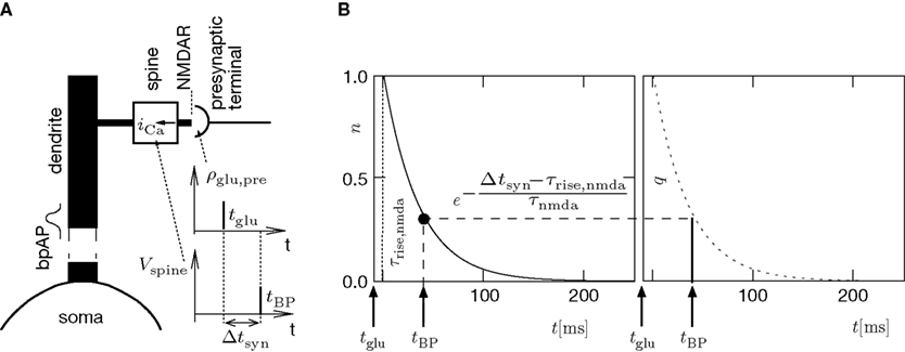
Figure 1. (A) Sketch of an experiment measuring the calcium concentration in spines during a spike pairing protocol. The calcium concentration inside the spine is measured while varying the temporal difference Δtsyn between the onset tglu of the glutamate concentration and the arrival of a postsynaptic bpAP tBP at the spine. (B) Rise in glutamate concentration at tglu in the synaptic cleft causes NMDA receptors in the spine to bind to glutamate. The fraction n(t) of glutamate bound NMDARs jumps to its maximum (n0 = 1 for simplicity) after time τrise,nmda. As long as the spine is not depolarized, the NMDA pore is blocked by Mg2+. A postsynaptic spikes causes a bpAP to arrive at the spine at tBP and to unblock the currently glutamate bound NMDA receptors n(tBP), so Ca2+ can enter the spine. The total amount of Ca2+ influx q is proportional to n(tBP) and therefore depends on the relative timing Δtsyn.
n(tBP) = n(tBP − tglu).
This is illustrated in Figure 1
B. Thus the NMDA receptor mediated conductivity depends on the relative timing Δtsyn = tBP − tglu. This model assumes instantaneous removal of the Mg2+ block. However, the detailed mechanism is more complicated. Removal of the Mg2+ block can happen at several time scales; a very fast one of 100 μs (Jahr and Stevens, 1990b
) and several recently found longer time scales of a few 100 ms (Kampa et al., 2004
). The longer time scales were found to effectively narrow the time window of substantial NMDA conductance (Kampa et al., 2004
). Here, we do not intend to capture the NMDA receptor kinetics in full detail, but rather to construct a functional yet quantitative model where the experimental results constrain the model parameters. Calcium imaging studies on spines (Nevian and Sakmann, 2004
) show, that the timing dependence of the Ca2+ peak amplitude can be fitted for positive Δtsyn to a function with a rise time of τrise,nmda followed by a exponential decay with a single time constant of τnmda. These studies typically measure the timing Δt = tpost − tpre between the spiking in the presynaptic neuron’s soma tpre and the spiking in the postsynaptic neuron’s soma tpost (see Morrison et al., 2008
, for the definition of delays in models of synaptic plasticity). With dBP being the delay for a bpAP and dglu being the delay between presynaptic spike and glutamate release, the timing difference at the synapse is
100 μs (Jahr and Stevens, 1990b
) and several recently found longer time scales of a few 100 ms (Kampa et al., 2004
). The longer time scales were found to effectively narrow the time window of substantial NMDA conductance (Kampa et al., 2004
). Here, we do not intend to capture the NMDA receptor kinetics in full detail, but rather to construct a functional yet quantitative model where the experimental results constrain the model parameters. Calcium imaging studies on spines (Nevian and Sakmann, 2004
) show, that the timing dependence of the Ca2+ peak amplitude can be fitted for positive Δtsyn to a function with a rise time of τrise,nmda followed by a exponential decay with a single time constant of τnmda. These studies typically measure the timing Δt = tpost − tpre between the spiking in the presynaptic neuron’s soma tpre and the spiking in the postsynaptic neuron’s soma tpost (see Morrison et al., 2008
, for the definition of delays in models of synaptic plasticity). With dBP being the delay for a bpAP and dglu being the delay between presynaptic spike and glutamate release, the timing difference at the synapse is
In this work, we neglect the continuous binding process and instead assume that the number n of glutamate bound NMDA receptors jumps to a positive value after the rise time τrise,nmda, like

where H(t) denotes the Heaviside function. Assuming the bpAP to be a point event, the total Ca2+ influx into the spine
depends exponentially on the timing Δt where iCa = q0δ(t − tBP) is the calcium current through a single open NMDA channel during a bpAP. Our expression for q defines the effective rise time τrise and suggests to measure q in units of q0n0, i.e. we set q0n0 = 1. Nevian and Sakmann (2004)
measured an effective rise time τrise = 10 ms and an exponential decay with a time constant τnmda = 32 ms.
The postsynaptic depolarization due to the AMPA receptor activation only causes a small NMDA conductivity, as shown in measurements of the NMDA conductivity for voltage patterns caused by spike pairing experiments (Kampa et al., 2004
) and also directly by observing that the calcium transient in spines in spike pairing experiments is not decreased significantly by blocking AMPA receptors (Nevian and Sakmann, 2004
). In our model, we neglect the influence of AMPA mediated depolarizations on the calcium signal.
Assuming the bpAP to be a point event is obviously an approximation. As well as the assumption, that the glutamate binding state jumps from 0 to 1 at t = tglu + τrise,nmda instead of showing a continuous increase on a time scale of 5–10 ms (as found experimentally by Kampa et al., 2004
). However, for timings Δtsyn ≥ τrise,nmda, it is easy to see that this does not qualitatively change the total Ca2+ influx (assuming iCa(t < 0) = 0, because
As before, q depends exponentially on the relative timing Δtsyn. The exact shape of the bpAP only enters the timing independent factor q′0. For Δtsyn < τrise,nmda, the integral depends both on the shape of the resulting iCa(t), which in turn depends on the actual shape of the bpAP, and on the rising flank of the NMDA channel activation. A typical trace of iCa(t) has a half duration of 5 ms and the rise time of NMDA activation is of the same order of magnitude (5–10 ms). Hence, the slope of q(Δtsyn) in this range is large compared to the following exponential decay with τnmda, as confirmed experimentally (Nevian and Sakmann, 2004
). The step like approximation (Eq. 2) therefore seems adequate. Our choice to describe the bpAP to be a point event has the consequence that in this spike pairing experiment there is no calcium influx for larger negative timings Δtsyn − τrise,nmda < 0. Taking into account a finite short decay time for the postsynaptic depolarization as in Shouval et al. (2002)
would lead to a small calcium influx also for the post-before presynaptic timing.
5 ms and the rise time of NMDA activation is of the same order of magnitude (5–10 ms). Hence, the slope of q(Δtsyn) in this range is large compared to the following exponential decay with τnmda, as confirmed experimentally (Nevian and Sakmann, 2004
). The step like approximation (Eq. 2) therefore seems adequate. Our choice to describe the bpAP to be a point event has the consequence that in this spike pairing experiment there is no calcium influx for larger negative timings Δtsyn − τrise,nmda < 0. Taking into account a finite short decay time for the postsynaptic depolarization as in Shouval et al. (2002)
would lead to a small calcium influx also for the post-before presynaptic timing.The Ca2+ influx q leads to a transient signal which in good approximation decays in an exponential fashion (Nevian and Sakmann, 2004
, 2006
; Waters et al., 2003
) with a decay time of 20–200 ms (reviewed in Cavazzini et al., 2005
). We therefore assume the calcium peak amplitude to depend linearly on the amount q of calcium influx.
Ca2+ Transients Caused by Correlated Irregular Spiking
So far we studied the model for the case of a spike pairing protocol, where a presynaptic action potential is paired with a postsynaptic action potential. In this section we investigate how much information about the correlation between presynaptic and postsynaptic events is contained in the Ca2+ signal if the spiking activity is irregular. To this end, we simulate the presynaptic and the postsynaptic spiking as Poisson processes with rates νi and νo, respectively. Both processes share a fraction of spikes that appear in the spike trains with a fixed temporal distance Δt. In the following we call these events “pair events”. Figure 2
A illustrates these processes. The strength of the temporal correlation is given by the correlation coefficient ε, which is the conditional probability of a pair event (i.e. seeing the temporally correlated presynaptic partner spike at t − Δt), given a postsynaptic spike at time t.
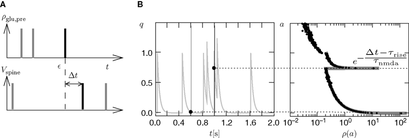
Figure 2. (A) Presynaptic glutamate release treated as point events ρglu,pre(t). The back-propagating action potentials cause a postsynaptic depolarization Vspine(t), taken to be point events as well. Pre- and postsynaptic events occur with Poisson statistics at ν = 5 Hz, but both sequences contain a fraction of correlated events (black bars), which have a fixed temporal distance Δt = 15 ms from each other. ε = 0.1 is the probability of observing a presynaptic partner, given a postsynaptic spike. The gray bars denote postsynaptic spikes, which have no correlated partner among the presynaptic events. (B) The left plot shows the shot noise (light gray) produced by the presynaptic events. A postsynaptic spike tpost samples the shot noise at the time of occurrence, a := q(tpost). Postsynaptic spikes that belong to a pair (i.e. which are preceded by a presynaptic event Δt before) are indicated by black bars. They sample q(t) at high values and thus produce the peak in the histogram (right panel) at  (with τrise = 5 ms). The black dots result from a realization of the stochastic process (T = 105 s) using Scientific Python (Jones et al., 2001
), the gray curve illustrates (Eq. 5). The peak amplitude is proportional to the correlation coefficient ε = 0.1. Uncorrelated postsynaptic events cause the peak at low values of a.
(with τrise = 5 ms). The black dots result from a realization of the stochastic process (T = 105 s) using Scientific Python (Jones et al., 2001
), the gray curve illustrates (Eq. 5). The peak amplitude is proportional to the correlation coefficient ε = 0.1. Uncorrelated postsynaptic events cause the peak at low values of a.Let A be the set of presynaptic spike times and B the set of postsynaptic spike times within a finite interval [0, T]. The effects of the presynaptic spikes add up linearly in our model. Therefore, the number of glutamate bound NMDA receptors found at time t is

and the total Ca2+ influx at the point in time tpost of a postsynaptic spike is accordingly
where we again set q0n0 to unity. For different realizations of the presynaptic and postsynaptic spiking the elements of the set aA,B = {qA(tpost) | tpost ∈ B} are random variables, since A and B are random sets. We therefore need to calculate the probability density function of qA and show that it depends on the correlation ε between pre- and postsynaptic events. Initially assume ε = 0, i.e. A and B to be two independent sets of Poisson points. In this case the points in time tpost at which qA(t) is sampled are randomly and uniformly drawn from the interval [0, T]. Consequently the elements a ∈ aA,B occur according to the probability density function of qA(t), where t is a randomly and uniformly drawn point in time t ∈ [0, T]. This is the amplitude distribution ρ0(q) of a shot noise with an exponential kernel and can be calculated recursively (Gilbert and Pollak, 1960
) as
where γ is Euler’s constant. In the case 0 < ε ≤ 1, however, we have to distinguish two cases: Given a postsynaptic spike, with probability 1 − ε this spike is not part of a pair event. The postsynaptic event is uncorrelated with respect to the presynaptic events and thus samples q(t) at a random point in [0, T] as discussed above. So the contribution of this event to the probability density ρ(a) is (1 − ε)ρ0(a). With probability ε the postsynaptic spike is part of a pair event. In this case, we know that there is a presynaptic spike at time tpost − Δt of which we still see the deterministic contribution  to a. Since we assume the presynaptic spikes to have Poisson statistics, the existence of the presynaptic spike at tpost − Δt does not influence the statistics of the other presynaptic spikes. The latter produce a shot noise background obeying the distribution ρ0(a′): the probability density to observe the value a = a′ + Δa equals the probability density ρ0(a′). Hence the contribution in this case is ερ0(a − Δa). Considering both types of postsynaptic spikes we arrive at
to a. Since we assume the presynaptic spikes to have Poisson statistics, the existence of the presynaptic spike at tpost − Δt does not influence the statistics of the other presynaptic spikes. The latter produce a shot noise background obeying the distribution ρ0(a′): the probability density to observe the value a = a′ + Δa equals the probability density ρ0(a′). Hence the contribution in this case is ερ0(a − Δa). Considering both types of postsynaptic spikes we arrive at

Figure 2
B illustrates this result. The postsynaptic events belonging to spike pairs (black bars) sample the shot noise signal at high values and cause the peak in the histogram around 0.73. Its height scales linearly with the correlation coefficient ε. The uncorrelated gray events cause a background manifested in the histogram by the large peak at low values. Its amplitude scales proportional to 1 − ε.
In conclusion, the information about correlation between the presynaptic and the postsynaptic events enters the probability distribution ρ(a) and is therefore exhibited in the amplitude distribution of Ca2+ transients in the postsynaptic spine: correlated postsynaptic events which come in close temporal proximity to a presynaptic spike produce a high Ca2+ influx.
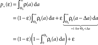
A Counter for Correlated Events
In this section we devise a model of a postsynaptically realized counter for correlated events. The model is based on CaMKII, the most probable downstream signaling protein. CaMKII is an example of a bistable effector protein, whose transitions between its active and its inactive state are triggered by distinct calcium concentrations. Since the number of CaMKII molecules in a spine is low a statistical description is essential. Figure 3
A shows a schematic drawing of the possible transitions of a single ring molecule in our model and their dependence on the calcium concentration: If the calcium influx exceeds the highest threshold Θh, the number x of active CaMKII molecules is increased. We call this a plus-event. If the influx is between Θl and Θh, the amount of active molecules remains unaffected. This region is often referred to as “no man’s land” (Cormier et al., 2001
). For a low calcium influx between Θb and Θl, the number of active molecules decreases. We call this a minus-event. If the influx is below Θb, the number of active molecules remains the same. Previous theoretical work (Shouval et al., 2002
) assumes a similar dependence of the synaptic weight change on the calcium concentration, but does not take into account the intermediate concentration, where no plasticity occurs. After a high calcium event, the concentration eventually drops to levels between Θb and Θl, where it can activate the phosphatase and thus deactivates CaMKII molecules. So the increase of active molecules in our model caused by a high Ca2+ event is understood to be the net effect of activated minus deactivated molecules.
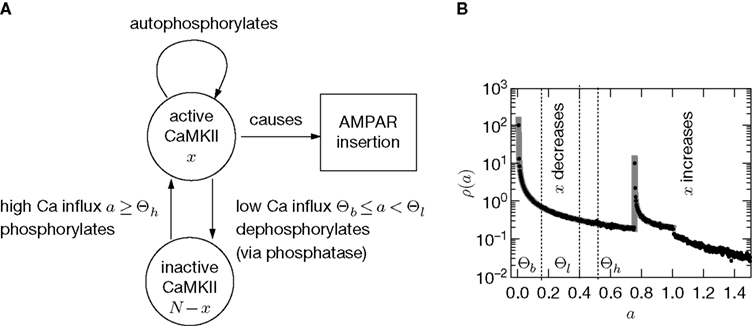
Figure 3. (A) CaMKII molecules exhibit bistability: An inactive state and a highly phosphorylated, active state. Transitions between the two states are triggered by Ca2+ influx. If the influx exceeds a threshold Θh, the molecule switches from inactive to active. Low Ca2+ influx between Θb and Θl deactivates the molecule. (B) At each postsynaptic spike, Ca2+ can enter the spine and can change the amount x of active CaMKII molecules. The probability density function ρ(a) of the Ca2+ influx at the points in time of a postsynaptic spike a = q(tpost) determines the direction of the effect on x (same data as in Figure 2
B). According to this effect, it can be divided into different regions: For Θb ≤ a < Θl; the number of active molecules is reduced. This event occurs with probability p− (Eq. 7). For a ≥ï Θh the number is increased, occurring which probability p+ (Eq. 6). In the regions between Θl and Θh and below Θb there is no influence on x.
Cormier et al. (2001)
measured the thresholds for constant calcium concentrations. It is unclear, whether these values also hold for transient calcium influx through NMDA receptors. Furthermore, for the spike pairing protocol, only relative calcium concentrations have been measured. We therefore pursue a more phenomenological approach and choose Θh such that a plus-event occurs, if the temporal distance between the presynaptic and the postsynaptic event Δt is in the range 0 ≤ Δt = tpost − tpre ≤ Δt+ = 20 ms, consistent with the potentiation window of STDP (Bi and Poo, 1998
). Furthermore, Bi and Poo (1998)
showed that the transition from LTD to LTP occurs in a relatively narrow time window symmetric around Δt = 0. Since in the present work we aim at a functional model we choose the effective rise time to be τrise = 0 ms, in order for the coincidence window to start at Δt = 0. Θh is then given by 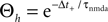 (see Figure 4
). Subsequently, we use the absolute values of Θh and Θl of Cormier et al. (2001)
to infer from the ratios
(see Figure 4
). Subsequently, we use the absolute values of Θh and Θl of Cormier et al. (2001)
to infer from the ratios  and
and  the appropriate values of Θl and Θb for our condition.
(see Figure 4
). Subsequently, we use the absolute values of Θh and Θl of Cormier et al. (2001)
to infer from the ratios and the appropriate values of Θl and Θb for our condition.
Figure 4. (A) Spike pairs with timing differences Δt ≤ Δt+ = 20 ms produce
plus-events. This determines the threshold  (B) Dependence of
  on the presynaptic rate νi for two different correlation coefficients ε = 0 (black) and for ε = 0.3 (gray). The maximum spike rate νi,max at which the detector can discriminate these two correlation coefficients results from the condition that s(ε) > s(0) for all νi ≤ νi,max.
(B) Dependence of on the presynaptic rate νi for two different correlation coefficients ε = 0 (black) and for ε = 0.3 (gray). The maximum spike rate νi,max at which the detector can discriminate these two correlation coefficients results from the condition that s(ε) > s(0) for all νi ≤ νi,max.Note that this choice of thresholds has the consequence for the spike pairing protocol that for 0 ≤ Δt ≤ Δt+ we obtain activation of CaMKII molecules, but we do not obtain deactivation for the reversed timing Δt < 0 as suggested by the experimentally observed LTD window of STDP. In the section “Sensitivity of Results to Model Assumptions” we discuss an extension of our model to incorporate the LTD window for negative relative timing and we argue that our results are invariant under this modification.
Knowing the probability distribution ρ(a) of the calcium peak amplitudes a given a postsynaptic depolarization, we can calculate the probability of occurrence p− = P(Θb ≤ a < Θl | postsynaptic spike) of a minus-event and p+ = P(a ≥ Θh | postsynaptic spike) of a plus-event. In order to detect pairs of correlated pre- and postsynaptic events, their relative timing must satisfy Δt ≤ Δt+. This is equivalent to the condition  , meaning, that correlated events cause an influx larger than Θh (compare Figure 3
B).
, meaning, that correlated events cause an influx larger than Θh (compare Figure 3
B).
, meaning, that correlated events cause an influx larger than Θh (compare Figure 3
B).Using Eqs. 5 and 4 for the probability of a plus-event we arrive at

Here r and C are given as in Eq. 4. An analogous calculation, which is valid under the same assumption Θb < Θl < Θh ≤ Δa yields
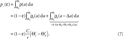
Each PSD of a spine contains a number of CaMKII molecules, which was found to be N = 80 in a typical PSD on average (Chen et al., 2005
). We are only interested in the behavior of the two stable states of a molecule: On long time scales, a molecule can only be in the fully activated or in the completely inactive state. Let the number of active molecules be x and assume that the postsynaptic neuron spikes with a rate νo. Then x is a random variable and we are interested in the equilibrium distribution and its dependence on the correlation between the presynaptic and postsynaptic spike train. Each postsynaptic spike may lead to a plus-event with probability p+(ε). In such an event, each of the N − x inactive molecules can become active. In our model, this transition happens independently for each particle with probability p. Given x active molecules, the number of molecules per time being activated is νo p + p(N − x). Analogously, the number of molecules per time being deactivated is νop−qx. Here, q is the probability of a minus-event to deactivate a particular molecules. This scenario is sketched in Figure 5
. In equilibrium, both currents must compensate, leading to the expected number of active molecules
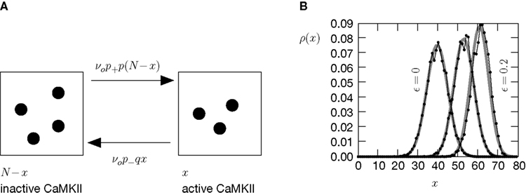
Figure 5. (A) Finite reservoir model of CaMKII. Each of the N = 80 molecules can either be active or inactive. Given a high calcium influx a ≥ Θh (which occurs with probability p+), each CaMKII molecule has the probability p = 0.01 to be activated. Given a low calcium influx Θb ≤ a < Θl (occurring with probability p−), the probability of an active molecule to be deactivated is q = 0.01. Presynaptic and postsynaptic events are Poisson with rates νi = νo = 5 Hz. The transition rates between the inactive and the active state are therefore νop+p(N − x) and νop−qx, respectively. (B) Equilibrium distribution of the number of active molecules x in an ensemble of synapses for different correlation coefficients ε = {0, 0.1, 0.2}. The activation rate increases with the correlation ε, whereas the deactivation rate decreases, shifting ρ(x) to the right. The black curves shows simulation results (temporal resolution 0.1 ms), the gray curves are Gaussians parameterized by
Eqs. 8 and 17.

Thus〈x〉eq depends on the relative probabilities p+(ε) for a plus-event and p−(ε) for a minus-event given by Eqs. 6 and 7. Figure 5
B shows the probability distribution for the number of active molecules for an ensemble of synapses, where the presynaptic and the postsynaptic activity are correlated Poisson processes. The higher the correlation coefficient ε between presynaptic and postsynaptic activity is, the more the distribution is shifted to the right. For a derivation of the first and second moment of the probability distribution see section “Probability Distribution for the Number of Active CaMKII Molecules” in Appendix.
The amount of active CaMKII molecules is the signal that can trigger downstream processes in the postsynaptic spine. Synapse maturation caused by insertion of new AMPA receptors into the PSD is such a process. In our model we assume that the process requires the presence of a certain minimal amount Xm of active CaMKII molecules. The probability of a synapse to maturate is therefore the probability that the number x of active molecules exceeds the threshold Xm. In a premature synapse, the initial Ca2+ concentration is low and hence the amount of active CaMKII is low as well. We would like to know the mean time needed by the signal x, starting at x = 0, to cross the threshold Xm for the first time. This is the mean first passage time problem. We approximate the mean first passage rate by the decay rate of the slowest decaying eigenvector of the CaMKII distribution in the section “Mean First Passage Time Problem for the Number of CaMKII Molecules” in Appendix. This solution is plotted for different thresholds in Figure 6
.
Figure 6. (A) Distribution  of the number of active molecules in an ensemble of synapses averaged over time. Synapses with x < Xd are pruned. This threshold acts as an absorbing boundary. Semi-analytic expression (Eq. 19) (gray), simulation of N = 10 000 synapses subject to presynaptic Poisson activity of νi = 5 Hz and postsynaptically the spiking activity of an integrate and fire neuron with νo = 9 Hz (black). (B) The number of surviving synapses as a function of time. Simulation (black) and analytical expectation value (gray) (Eq. 29). The death rate (slope) corresponds to the eigenvalue η1. Different rates are obtained for the thresholds Xd = 25, 30, 35, where the fastest decay belongs to the highest threshold Xd = 35. (The parameters of the integrate and fire neuron are: membrane time constant τm = 20 ms, threshold Vth = 15.0 mV,, reset potential Vr = 0 mV. It receives excitatory Poisson input of νext = 35400 Hz from synapses with weight w = 0.05 mV and inhibitory Poisson inputs of rate νinh = 5600 Hz from synapses of weight −gw = −0.2 mV.)
of the number of active molecules in an ensemble of synapses averaged over time. Synapses with x < Xd are pruned. This threshold acts as an absorbing boundary. Semi-analytic expression (Eq. 19) (gray), simulation of N = 10 000 synapses subject to presynaptic Poisson activity of νi = 5 Hz and postsynaptically the spiking activity of an integrate and fire neuron with νo = 9 Hz (black). (B) The number of surviving synapses as a function of time. Simulation (black) and analytical expectation value (gray) (Eq. 29). The death rate (slope) corresponds to the eigenvalue η1. Different rates are obtained for the thresholds Xd = 25, 30, 35, where the fastest decay belongs to the highest threshold Xd = 35. (The parameters of the integrate and fire neuron are: membrane time constant τm = 20 ms, threshold Vth = 15.0 mV,, reset potential Vr = 0 mV. It receives excitatory Poisson input of νext = 35400 Hz from synapses with weight w = 0.05 mV and inhibitory Poisson inputs of rate νinh = 5600 Hz from synapses of weight −gw = −0.2 mV.)We treat synapse pruning analogously. In a mature synapse the initial amount of active CaMKII is already beyond the threshold Xm. Due to pre- and postsynaptic activity, the amount x of active CaMKII may decrease or increase, depending on the rates and the pre- and postsynaptic correlation. If eventually x falls below the minimal amount Xd, the synapse dies. We choose Xd < Xm for two reasons. First, once the amount of CaMKII is high, autophosphorylation will act regeneratively (Miller et al., 2005), making the decrease of x harder. We do not model this dynamics explicitly, but rather incorporate its effect in our choice of Xd < Xm. Secondly, experiments by Le Be and Markram (2006)
suggest, that there is a “period of grace” for newly formed synapses during which they are not pruned, preventing many synapses to be created and destructed in vain. Our choice is a possible implementation.
Rate Homeostasis by Synaptic Pruning
In this section we employ the correlation detection mechanism to control synaptic pruning and demonstrate its capability to regulate spike rate towards a state of low rate. Before doing so we generalize the correlation model studied in previous sections to the more realistic scenario of a temporally extended correlation between the presynaptic and the postsynaptic activity.
The correlation detection depends on the probabilities p+ for a plus-event (high Ca2+ influx) and p− for a minus-event (low Ca2+ influx). A plus-event happens, whenever the influx a is in the range a ≥ Θh. In order to compute p+ and analogously p− we need to specify the pair correlation function Cio(t1, t2) between the presynaptic and the postsynaptic spike train. Generally, the correlation function is defined as
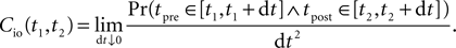
Here we restrict ourselves to stationary processes, such that Cio(t1, t2) = Cio(t2 − t1) only depends on the relative timing τ = t2 − t1 between the presynaptic and the postsynaptic spike. Furthermore, we assume the presynaptic spikes to be Poisson events emitted at rate νi. The postsynaptic spikes appear with mean rate νo. For large τ the cross-correlation function decays to 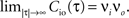 Hence we can write
Hence we can writeCio(τ) = νiνo + cio(τ),
where the cross-covariance cio vanishes for large |τ|. We now know the conditional probability to observe a presynaptic spike at tpre ∈ [t − τ, t − τ + dt] provided that a postsynaptic spike occurs at time t

For a presynaptic spike to cause a plus-event it must have appeared within the potentiation window (see Figure 4
A), i.e. 0 ≤ τ ≤ Δt+. So the correlation detector measures the probability εeff exceeding chance level of finding a presynaptic spike within this potentiation window, given a postsynaptic event at t = 0. This probability is 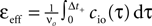 . The cross-covariance cio(τ) decreases on a time scale comparable to the membrane time constant of the neuron, which is typically shorter than the potentiation window Δt+ = 20 ms. An example can be seen in Figure 7
A. In this case we can make the simplification
. The cross-covariance cio(τ) decreases on a time scale comparable to the membrane time constant of the neuron, which is typically shorter than the potentiation window Δt+ = 20 ms. An example can be seen in Figure 7
A. In this case we can make the simplification
. The cross-covariance cio(τ) decreases on a time scale comparable to the membrane time constant of the neuron, which is typically shorter than the potentiation window Δt+ = 20 ms. An example can be seen in Figure 7
A. In this case we can make the simplification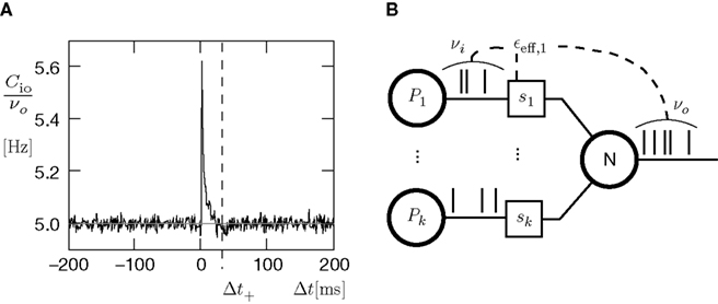
Figure 7. (A) Input–output correlation function normalized to the postsynaptic spike rate. The peak drops to baseline (νi = 5 Hz, gray) on a time scale which is shorter than the width of the potentiation window Δt+ = 20 ms. The area below the peak is the effective correlation coefficient εeff (see Eq. 10). (B) A neuron
N receiving k Poisson spiking inputs of rate νi = 5 Hz via synapses s1…sk. Each synapse measures the correlation between its input spike train and the spiking activity of the neuron N. A synapse is pruned as soon as its number of active CaMKII has fallen below a threshold x < Xd = 30.

The probabilities of plus and minus-events are then given by Eqs. 6 and 7, respectively, with ε = εeff . An analytic approximation for the effective correlation coefficient in the framework of linear response theory for an integrate and fire neuron model can be found in the section “Input Output Correlation of an Integrate and Fire Neuron” in Appendix. Note that the causal dependence of output spikes on the input spikes and the assumed Poisson statistics of the incoming activity leads to the input–output correlation function (Figure 7
A) which only deviates from baseline for Δt > 0. Therefore, the position of the temporal window for minus events is uncritical in this setup, as long as cio is at baseline within this window. Thus we would obtain the same results, if the time window for minus events was at negative times.
We now have the tools to investigate synaptic pruning in the scenario depicted in Figure 7
B. A neuron initially has a number k0 of synaptic excitatory inputs, each of which reaches the neuron via a spiny synapse with a calcium based correlation detector as described in the section “A Counter for Correlated Events” All synapses are mature and may eventually die depending on the correlation variable x: A synapse is pruned as soon as the amount x of active CaMKII undercuts a critical threshold x < Xd. The initial distribution of x over the ensemble of synapses is the eigenvector of the slowest decaying eigenmode at the initial firing frequency νo(0) of the neuron. The choice is justified, if we think of the initial connectivity as the outcome of a slow dynamic wiring process, during which the synaptic amount x of active CaMKII had enough time to settle in this eigenmode. In addition to the excitatory inputs, the neuron receives a static configuration of inhibitory connections. Due to the pruning process, excitatory synapses progressively die and hence the number of excitatory connections k(t) decays and the neuron’s firing rate νo decreases (see Figures 8
A,B). The pruning process continues until the postsynaptic neuron stops spiking. Thus, pruning is a mechanism to regulate the firing rate downwards. If the process is slow compared to the dynamics of x, we can assume the distribution of x to follow the eigenstate adiabatically. In this approximation, the development of connectivity obeys the differential equation
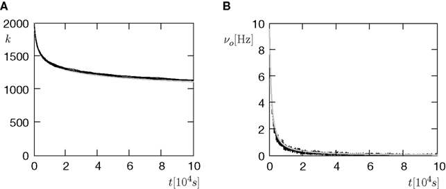
Figure 8. (A) The number of incoming connections (vertical) in the course of the pruning process of Figure 7
B. (B) The firing rate of the neuron (vertical) reduces with the reduction of inputs (A). Black: five simulation trials. Gray: Numerical integration of Eq. 11. Initial number of incoming connections k0 = 2000. In addition, the neuron receives 5080 excitatory connections and 1120 inhibitory connections, which are not pruned.
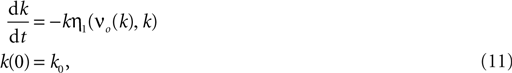
where η1(νo, k) is the eigenvalue of the slowest decaying eigenmode. All terms are accessible: a derivation of η1 is presented in the section “Mean First Passage Time Problem for the Number of CaMKII Molecules” in Appendix and νo can be calculated using Eq. 34. Therefore, Eq. 11 can be numerically integrated. Figure 8
compares this semi-analytic result with a direct simulation of the model.
The negative slope of the pruning curve in Figure 8
A is decreasing with decreasing number of incoming synapses k. The reason is the dependence of the synapse death rate on the postsynaptic firing rate: The time scale of activation and deactivation of the CaMKII molecules is determined by the postsynaptic firing rate νo (compare Eq. 20). Consequently, also the death rate is proportional to νo. This is an interesting feature, since it facilitates a firing rate homeostasis: If new synapses are created with a constant rate the input connectivity to the neuron has a stable fixed point at k* where synaptic death is just compensated by synapse creation. The firing rate of the neuron assumes a corresponding fixed firing rate ν*o. A similar example of such a homeostasis will also be shown in the section “Synaptic Maturation and Pruning”.
Cooperation and Competition by Spatial Input Correlation
In the previous section we investigated a synaptic pruning process, where all excitatory inputs are uncorrelated. However, there is evidence that coactive inputs are stabilized (Cohen-Cory, 2002
) and therefore less likely to be pruned. Here we show, that the calcium based correlation detection mechanism naturally leads to cooperation between synapses, which stabilizes coactive inputs.
Synaptic Pruning
In the first setup, we investigate a neuron receiving excitatory inputs from two different sources: A pool of np presynaptic neurons with uncorrelated Poisson spiking activity at rate νi. We call these inputs the “independent inputs” in the following. The second pool of nc Poisson spiking neurons at rate νi, however, generates correlated spike trains. We use the multiple interaction process (Kuhn et al., 2003
) to produce the spike trains and call these the “correlated inputs”. The correlation coefficient 0 < c ≤ 1 is the probability of input neuron i having an input spike at time t, given neuron j has a spike at the same time. Thus, c = 0 results in uncorrelated Poisson processes, whereas for c = 1 all nc spike trains are the same.
Initially (at t = 0) there are np(0) = nc(0) = 1000 incoming synapses. Each of the synapses uses the calcium based correlation detection mechanism to determine the number of active CaMKII molecules x. Whenever x falls below the threshold Xd, the corresponding synapse dies. Figure 9
A illustrates this scenario.
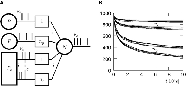
Figure 9. (A) A neuron receiving two pools of excitatory inputs: np synapses provide uncorrelated Poisson inputs at νi = 5 Hz, and nc synapses correlated Poisson inputs at rate νi = 5 Hz. The correlated events are produced by the multiple interaction process parameterized by the pairwise correlation c. A continuous pruning process eliminates synapses when the number of active CaMKII falls below a threshold x < Xd = 30. (B) Evolution of connectivity structure. Initially, both groups have the same number of synapses np(0) = nc(0) = 1000. In addition, the neuron receives 5080 excitatory connections and 1120 inhibitory connections, which are not pruned. The pruning process mainly affects the uncorrelated inputs. The top and the bottom trace are for a pair correlation c = 0.01, the intermediate traces for c = 0.005. Black: five simulation trials. Gray: Numerical integration of Eq. 12.
Figure 9
B shows the evolution of the number of incoming connections. The synapses from independent sources exhibit a higher death rate than synapses from correlated inputs. We can readily understand this behavior: Given there is a spike at input i of the correlated pool, each of the remaining nc − 1 inputs also delivers a spike with probability c at the same time. Thus, given a spike at the correlated input i, the expectation value for the sum of all inputs at this time is 〈w〉mip = w(1 + c(nc − 1)), where w is the homogeneous synaptic weight. In contrast, a spike from the uncorrelated pool only carries its own weight w < 〈w〉mip. A higher synaptic weight results in a higher probability of the target neuron to emit a spike. Thus, the probability of the neuron to fire in response to a spike from one of the correlated inputs is higher than for an uncorrelated input. This probability is proportional to the correlation coefficient εeff between the presynaptic and the postsynaptic spike train (for a derivation of an analytic expression for εeff see Eq. 37 in the section “Correlated Poisson Input” in Appendix). With εeff,mip > εeff,Poisson, the number of active molecules x in the synapses from correlated inputs is higher than in those from independent inputs (see also Figure 5
B) and hence their death rate is lower (see also “A Counter for Correlated Events”).
Although there is no direct interaction between synapses from correlated inputs, cooperativity emerges between them and helps to stabilize these inputs in favor of the uncorrelated inputs. There is not only cooperation among synapses of the correlated pool, but also competition between the two pools: The number of uncorrelated inputs decreases with increasing correlation among the correlated inputs. This is because the synaptic deathrate increases with the firing rate of the target neuron.
The time evolution of the number of inputs np(t) and nc(t) can be calculated numerically completely analogous to the section “Rate Homeostasis by Synaptic Pruning”. The system of differential equations governing the dynamics is
where η1,Poisson(νo, np, nc) and η1,mip(νo, np, nc) are the slowest decaying eigen-modes calculated according to the section “Mean First Passage time Problem for the Number of CaMKII Molecules” in Appendix.
Synaptic Maturation and Pruning
In this section, we extend the scenario of Figure 9
A by incorporating a process of synapse creation. Again we have two pools of input neurons: The first pool of Np neurons has Poisson spiking activity with rate νi, the second pool of Nc neurons has Poisson activity with pair correlation c and the same rate νi. Excitatory synapses from both pools can exist in either of two states, premature or mature as depicted in Figure 10
A. Newly created synapses are in the premature state, lacking AMPA receptors. Their synaptic weight is 0. A synapse becomes mature, if the number of active molecules x exceeds a threshold Xm. The mature synapse has the synaptic weight w > 0. This synapse dies, if the number of active molecules falls below a threshold Xd. Initially there are no premature synapses np,pre(0) = nc,pre(0) = 0, and there are as many mature synapses from independent inputs as from correlated inputs np,mat(0) = nc,mat(0) > 0. Premature synapses are constantly created: For each of the Np − np,mat − np,pre presently unestablished connections from independent sources, the rate of realization is λpre. Premature synapses from correlated sources are created analogously with the same rate λpre.
Figure 10. (A) Each synapse has two states: In the premature state, its synaptic weight is w = 0. If the number x of active CaMKII exceeds a threshold Xm = 45, the synapse maturates and exhibits a synaptic weight w = 0.05 mV. If x falls below Xd = 30, the synapse dies. (B) Formation of input structure of a neuron during constant creation of premature synapses with rate  synapses per second in otherwise the same input scenario as in Figure 9
A. Initially, there are np,mat(0) = nc,mat(0) = 3540 mature excitatory synapses from each input pool and np,pre(0) = nc,pre(0) = 0 premature synapses. Additionally, there are inputs from 1120 inhibitory synapses not subject to pruning. The traces show (top to bottom): mature synapses from correlated pool nc,mat, mature synapses from uncorrelated pool np,mat, premature synapses from uncorrelated pool np,pre, premature synapses from correlated pool nc,pre. Black: simulation, gray: analytical approximation.
synapses per second in otherwise the same input scenario as in Figure 9
A. Initially, there are np,mat(0) = nc,mat(0) = 3540 mature excitatory synapses from each input pool and np,pre(0) = nc,pre(0) = 0 premature synapses. Additionally, there are inputs from 1120 inhibitory synapses not subject to pruning. The traces show (top to bottom): mature synapses from correlated pool nc,mat, mature synapses from uncorrelated pool np,mat, premature synapses from uncorrelated pool np,pre, premature synapses from correlated pool nc,pre. Black: simulation, gray: analytical approximation.The evolution of the connectivity in the presence of maturation and pruning is shown in Figure 10
B. The connectivity approaches an equilibrium state after t 600 s. The number of mature synapses from correlated inputs nc,mat increases, while the number of synapses from uncorrelated inputs np,mat decreases (upper two traces). The two values saturate at different levels, such that nc,mat > np,mat. Initially, the number of premature synapses increases for both input pools (lower two traces). In equilibrium, the numbers of premature synapses saturate at different levels np,pre > nc,pre. The explanation for this observation is the same as in the previous subsection: Correlatedly activated synapses exhibit cooperation, they experience a higher correlation coefficient between the input spike train and the output spike train produced by the neuron. Hence, for synapses from the correlated pool, the maturation rate of premature synapses is higher and the deathrate of mature synapses is lower as compared to the uncorrelated inputs. As in the section “Synaptic Pruning”, the target neuron becomes selective for the correlated pool.
600 s. The number of mature synapses from correlated inputs nc,mat increases, while the number of synapses from uncorrelated inputs np,mat decreases (upper two traces). The two values saturate at different levels, such that nc,mat > np,mat. Initially, the number of premature synapses increases for both input pools (lower two traces). In equilibrium, the numbers of premature synapses saturate at different levels np,pre > nc,pre. The explanation for this observation is the same as in the previous subsection: Correlatedly activated synapses exhibit cooperation, they experience a higher correlation coefficient between the input spike train and the output spike train produced by the neuron. Hence, for synapses from the correlated pool, the maturation rate of premature synapses is higher and the deathrate of mature synapses is lower as compared to the uncorrelated inputs. As in the section “Synaptic Pruning”, the target neuron becomes selective for the correlated pool.A similar differential equation as Eq. 12 quantitatively describes the evolution of the connectivity in this model. Its numerical solution (Figure 10
B, gray) corresponds well to a direct simulation of the system (black). The observed deviations are due to synapse maturation: Each synapse entering the mature state has a number x of active CaMKII just above threshold Xm. This perturbs the equilibrium distribution of x for the mature synapses and hence influences their death rate. The direction of this influence depends on the relative position of Xm with respect to the equilibrium
〈x〉eq: For Xm > 〈x〉eq the observed death rate is lower than the analytic estimate and vice versa.
In the present work we describe a novel model of the synaptic mechanisms controlling synapse pruning and synapse maturation. To our knowledge, this is the first model of structural plasticity based on the microscopic dynamics of the single synapse. Instead of constructing a phenomenological model, we use recent experimental findings to identify plausible postsynaptic mechanisms and to constrain the choice of model parameters. We analyze the cortical scenario of irregular spiking activity and quantify the dependence of structural plasticity on the correlation between the presynaptic and the postsynaptic activity. Functionally, the dynamics acts as a Hebbian learning rule for synaptogenesis and pruning. Our model can be understood as a biological plausible implementation of a cascade synapse (Rubin and Fusi, 2007
) for spiking activity, where the number x of active CaMKII molecules plays the role of internal states. However, in contrast to the cascade model, once x falls below the critical threshold the synapse is lost and cannot be reactivated by subsequent potentiating events. Here we provide a full statistical treatment of the number of active molecules. This is essential, since due to the low number of molecules (N 80) fluctuations cannot be neglected. Previous work on STDP (Cai et al., 2007
; Shouval and Kalantzis, 2005
) demonstrated, that stochastic fluctuations can change the phenomenology of a learning rule.
80) fluctuations cannot be neglected. Previous work on STDP (Cai et al., 2007
; Shouval and Kalantzis, 2005
) demonstrated, that stochastic fluctuations can change the phenomenology of a learning rule.We show that there are two distinct rate regimes: In the low rate regime up to νi 10 Hz, our model works as a correlation detector in the sense that synchronously activated synapses on the same dendrite stabilize. This frequency limit is a direct consequence of the NMDA unbinding time constant τnmda. Hence the model constitutes a viable mechanism for a network using temporal (correlation) codes at low rates. At higher rates (νi > 10 Hz), synapse stabilization occurs irrespective of correlations between input and output. This is in accordance with recent experimental evidence that higher activity leads to increased synapse formation (Le Be and Markram, 2006
) and to classical LTP induced by tetanic stimulation protocols. Furthermore, we show that by controlling synaptic pruning our model exhibits several desirable features for a neuronal network: The synaptic pruning rate increases with the postsynaptic firing rate. This enables the homeostasis of firing rate while synapses are continuously created, a finding obtained earlier using abstract rate based models of structural plasticity (van Ooyen et al., 1995
). Moreover, the synapses targeting the same neuron naturally exhibit cooperation and competition. These emerging phenomena render the proposed microscopic mechanism relevant for the theory of learning in neuronal networks: The evolution of connectivity is sensitive to correlations in the inputs and hence neurons become selective for coactive inputs. This stabilization of coactive inputs has been proposed earlier based on experimental evidence, reviewed in (Cohen-Cory, 2002
). Our treatment explains, how cooperation and competition are mediated solely by the identical postsynaptic activity experienced by synapses. Previous theoretical work (Kempter et al., 1999
, 2001
) showed cooperativity to emerge from the interplay of spike timing dependent learning rules with the spiking dynamics in the framework of spike response models. In general, a quantitative understanding of the interaction between a spike timing based plasticity rule and the integrate-and-fire dynamics is a hard problem. Here we provide such an analysis for our specific learning rule assuming all-to-all spike interaction. The analysis allows us to obtain semi-analytic expressions for the evolution of network structure. Specifically, we present results for the case of incoming irregular Poisson activity as well as for the case of correlated inputs generated by a multiple-interaction-process (Kuhn et al., 2003
).
10 Hz, our model works as a correlation detector in the sense that synchronously activated synapses on the same dendrite stabilize. This frequency limit is a direct consequence of the NMDA unbinding time constant τnmda. Hence the model constitutes a viable mechanism for a network using temporal (correlation) codes at low rates. At higher rates (νi > 10 Hz), synapse stabilization occurs irrespective of correlations between input and output. This is in accordance with recent experimental evidence that higher activity leads to increased synapse formation (Le Be and Markram, 2006
) and to classical LTP induced by tetanic stimulation protocols. Furthermore, we show that by controlling synaptic pruning our model exhibits several desirable features for a neuronal network: The synaptic pruning rate increases with the postsynaptic firing rate. This enables the homeostasis of firing rate while synapses are continuously created, a finding obtained earlier using abstract rate based models of structural plasticity (van Ooyen et al., 1995
). Moreover, the synapses targeting the same neuron naturally exhibit cooperation and competition. These emerging phenomena render the proposed microscopic mechanism relevant for the theory of learning in neuronal networks: The evolution of connectivity is sensitive to correlations in the inputs and hence neurons become selective for coactive inputs. This stabilization of coactive inputs has been proposed earlier based on experimental evidence, reviewed in (Cohen-Cory, 2002
). Our treatment explains, how cooperation and competition are mediated solely by the identical postsynaptic activity experienced by synapses. Previous theoretical work (Kempter et al., 1999
, 2001
) showed cooperativity to emerge from the interplay of spike timing dependent learning rules with the spiking dynamics in the framework of spike response models. In general, a quantitative understanding of the interaction between a spike timing based plasticity rule and the integrate-and-fire dynamics is a hard problem. Here we provide such an analysis for our specific learning rule assuming all-to-all spike interaction. The analysis allows us to obtain semi-analytic expressions for the evolution of network structure. Specifically, we present results for the case of incoming irregular Poisson activity as well as for the case of correlated inputs generated by a multiple-interaction-process (Kuhn et al., 2003
).Sensitivity of Results To Model Assumptions
For analytical convenience we use an integrate and fire neuron model with δ-shaped postsynaptic currents, as commonly used in network simulations and theoretical works. These currents can cause an immediate spiking response to an incoming spike. More realistic neuron models have postsynaptic currents with finite rise times and hence also the input–output correlation function shows a finite latency of τresponse 5 ms in response to an input spike. Since we aim at a consistent theory of the interaction between learning rule and neuronal dynamics, we compensate for the lack of latency by reducing the measured glutamate binding time τrise 5…10 ms to τrise = 0 ms. As in the natural setting the whole mass of the input–output correlation function falls into the time window τ+ of the learning rule. A mismatch of the time constants would not change the observed phenomena qualitatively, but slightly reduce the sensitivity to correlations. We can extend our analysis to more realistic and more complicated neuron models, if an expression for the corresponding integral input–output correlation  is known.
5 ms in response to an input spike. Since we aim at a consistent theory of the interaction between learning rule and neuronal dynamics, we compensate for the lack of latency by reducing the measured glutamate binding time τrise 5…10 ms to τrise = 0 ms. As in the natural setting the whole mass of the input–output correlation function falls into the time window τ+ of the learning rule. A mismatch of the time constants would not change the observed phenomena qualitatively, but slightly reduce the sensitivity to correlations. We can extend our analysis to more realistic and more complicated neuron models, if an expression for the corresponding integral input–output correlation is known.The probabilities p and q for activation and deactivation of CaMKII molecules by large and small calcium events respectively, are set to p = q = 0.01 without experimental reference. Once experimental data are available, these parameters need to be reconsidered. The smaller the values, the narrower the distribution of active CaMKII molecules. This increases the sensitivity to correlation but also the latency of the distribution in following transient changes in the correlation. The threshold Xd for the minimum number of active CaMKII molecules required for survival can be chosen such that the synapse turnover in a neuronal network reaches experimentally observed values of 7% of all synapses per week (Stettler et al., 2006
). As soon as an experimental value for Xd is available we can check whether our model consistently relates the two experimental measures. We use a multiple interaction process to generate incoming spiking activity with higher order correlations. The choice is motivated by analytical convenience rather than by biological realism. However, we expect other models of higher order correlation to exhibit qualitatively similar results for cooperation and competition between synapses.
Due to our assumption of a point event like bpAP (see also “Spike Time Dependence of Postsynaptic Calcium Concentration”) there is no calcium influx through NMDA receptors, if the postsynaptic depolarization precedes the presynaptic release of glutamate. For our model the consequence is that post-before-pre pairings do not cause deactivation of CaMKII molecules (see also “A Counter for Correlated Events”). Hence if the intention was to explain STDP, we would not be able to reproduce the part of the rule expressing LTD. Experimentally, Nevian and Sakmann (2004) observe calcium influx through NMDA receptors only for the pre-before-post condition. Additionally, there is influx through voltage dependent calcium channels (VDCC) opened by the bpAP. Also AMPA receptors depolarize the spine and hence lead to calcium entry through coactivated NMDA receptors and VDCCs. However, the resulting NMDA conductivity is small (Kampa et al., 2004
) and calcium transients in spines are not significantly decreased by blocking AMPA receptors (Nevian and Sakmann, 2004
). So here we assume the main pathway for calcium influx into the spine to be NMDA receptors and we neglect the additional sources of calcium. As long as their contribution to the calcium signal is small, they constitute a background elevation of the overall calcium level in the spine and we obtain qualitatively similar results. If, however, their contributions were of comparable size as the calcium transient through NMDA receptors, a temporally close post-before-pre timing could lead to sufficient calcium influx to deactivate CaMKII and hence create a LTD window. Previous biophysical models of STDP (Shouval et al., 2002
) assumed a finite decay time for the postsynaptic depolarization. This as well leads to an intermediate calcium influx for the post-before-pre condition. Our model can be extended in the same way. However, as argued in the section “Rate Homeostasis by Synaptic Pruning”, for the results presented here, the exact temporal position of the LTD window is irrelevant. The observed rate homeostasis only depends on the proportionality between the synapse death rate and the postsynaptic firing rate, resulting from the CaMKII dynamics. The cooperativity between synapses (see “Cooperation and Competition by Spatial Input Correlation”) only requires a Hebbian type plasticity, i.e. plus events are caused by a postsynaptic spike following a presynaptic spike in close succession.
Scope and Accuracy of the Analytical Treatment
The treatment of the CaMKII dynamics as a Markov process implicitly assumes the high (plus) and low (minus) calcium events to occur uncorrelatedly with the respective probabilities p+ or p−. However, the occurrence of a plus event or a minus event depends on the current value n(tpost), the fraction of glutamate bound NMDA receptors at the time of the postsynaptic spike. n(t) has a time constant τnmda = 32 ms. Hence, if postsynaptic spikes occur with arbitrarily small inter-spike-intervals, the probability to observe a plus event is slightly higher after a previous plus event. Nevertheless, for realistic postsynaptic spike trains, small inter-spike-intervals are rare due to refractoriness, so the neglect of the temporal correlation of n(t) is well justified (see also section “Mean First Passage Time Problem for the Number of CaMKII Molecules” in Appendix, Figure 12
B). A more thorough treatment must take into account the actual auto-correlation function of the postsynaptic spiking activity. The dynamics of the discrete amount of active CaMKII molecules is mapped to a continuous system. By comparing the continuous analytic probability density to the discrete numerical solution of the probability mass function, we found that this approximation is sufficiently accurate as long as the total number of molecules is large enough (N > 30). Furthermore, we approximate the CaMKII dynamics as a diffusion with a x-independent diffusion constant, whereas the original problem leads to a x-dependent diffusion term. Again, the nearly perfect agreement of the numerical solution (taking into account x-dependent diffusion) with the analytically obtained Gaussian, proves this approximation adequate (see Figure 11
). However, if the distribution approaches the saturation limits x = 0 or x = N, we observe pronounced deviations. This may occur for highly correlated spiking and at excessive firing rates. The results for the synaptic death and maturation rates are based on the slowest decaying eigenvalue η1 of the CaMKII activation distribution. This component has the largest time constant. If the ensemble of synapses is initialized with a distribution containing contributions different from the slowest decaying eigenvector, we observe transient deviations in the pruning rate. These transients decay typically 15 times faster than the slowest eigenvector  So after a sufficiently long time, the CaMKII distribution obeys the analytical solution in good approximation. For calculating the equilibrium state of connectivity, the slowest decaying eigenvector is the exact description if the number x of active molecules of a new synapse is drawn from this eigenvector. But even for non-stationary connectivity, the distribution of activated CaMKII across synapses follows the structure quasi adiabatically and the approximation is well fulfilled as shown by comparing analytical results with direct simulations (see “Rate Homeostasis by Synaptic Pruning” and “Cooperation and Competition by Spatial Input Correlation”). The larger deviations in Figure 10
are attributed to this approximation: Each synapse entering the mature state has a number x of active CaMKII just above threshold Xm. This perturbs the equilibrium distribution, explaining the deviation of the simulated from the analytically obtained connectivity structure.
So after a sufficiently long time, the CaMKII distribution obeys the analytical solution in good approximation. For calculating the equilibrium state of connectivity, the slowest decaying eigenvector is the exact description if the number x of active molecules of a new synapse is drawn from this eigenvector. But even for non-stationary connectivity, the distribution of activated CaMKII across synapses follows the structure quasi adiabatically and the approximation is well fulfilled as shown by comparing analytical results with direct simulations (see “Rate Homeostasis by Synaptic Pruning” and “Cooperation and Competition by Spatial Input Correlation”). The larger deviations in Figure 10
are attributed to this approximation: Each synapse entering the mature state has a number x of active CaMKII just above threshold Xm. This perturbs the equilibrium distribution, explaining the deviation of the simulated from the analytically obtained connectivity structure.
Figure 11. Comparison between the numerically obtained distribution of the number of active molecules in an ensemble of synapses solving Eq. 14 (black dotted curve) and the Gaussian approximation (gray curve) using Eqs. 16 and 17 for different pair correlation coefficients ε = {0, 0.1, 0.2} between the presynaptic and the postsynaptic spiking activity. Same parameters as in Figure 5
.
Figure 12. (A) Exit probability pexit given a minus-event depending on the state x (black) and probability density function ρ (gray) of the number of active molecules x. (B) Probability of having k consecutive plus-events given at least one plus-event. Expected probability 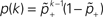 for independently occurring events (gray). Statistics of events caused by a postsynaptic spike train of an integrate and fire neuron (black dashed line) and of events caused by a postsynaptic Poisson spike train (black dashed-dotted line).
for independently occurring events (gray). Statistics of events caused by a postsynaptic spike train of an integrate and fire neuron (black dashed line) and of events caused by a postsynaptic Poisson spike train (black dashed-dotted line).Functional Role of Structural Plasticity
Recent experiments (Stettler et al., 2006
) demonstrated synaptogenesis and synaptic death to occur even in the adult cortex. However, their functional relevance for the neural network still remains to be illuminated. Theoretical considerations (Chklovskii et al., 2004
; Stepanyants et al., 2002
) suggest rewiring in networks to provide the dominating substrate of information storage. In artificial neural networks optimization of wiring was already shown to contribute significantly to memory capacity (Knoblauch, 2006
; Knoblauch et al., 2007
). More generally, restructuring of connectivity allows biological systems to optimize their circuitry to fulfill a specific set of functions. Understanding the mechanisms of wiring optimization will also be beneficial for technical systems (e.g. integrated circuits), since due to their essentially two dimensional nature, the number of contacts existing at any point in time is a precious and limited resource. For the above purposes a phenomenological model of structural plasticity is sufficient. However, a microscopic model is required to uncover the underlying biological mechanisms and resulting limitations. Moreover, an understanding of the control mechanisms of connectivity may contribute to the development of medical protocols to promote plasticity after neural lesions, e.g. as experienced after a stroke. How a system can exhibit a plastic structure and yet acquire and maintain its functionality is still a matter of research. To answer this question it is not sufficient to investigate synaptogenesis and synaptic death under conditions of stationary activity, but we rather have to consider the close interplay between the structural dynamics and the correlation dynamics exposed by the present work. The framework presented here provides the tools for this endeavor; we are now in the position to investigate structural plasticity in recurrent neural networks.
Probability Distribution for the Number of Active Camkii Molecules
Suppose there is a finite amount of CaMKII in the PSD. Each of the N molecules can either be active or inactive. Transitions between these states are triggered by calcium influx, where a high calcium amplitude a ≥ Θh causes each inactive molecule to be activated with probability p, and a low calcium amplitude Θb ≤ a < Θl causes each active molecule to be inactivated with probability q. The rate of high calcium events is λ+ = νo p+(ε), the rate of low calcium events λ− = νo p−(ε), where νo denotes the postsynaptic firing rate. Given x active molecules, the number of molecules being activated per time is λ+p(N − x), the current of molecules being deactivated is λ−qx. Since these rates depend on the state x of the system, the process has the Markov property. Thus, the system is uniquely defined by the transition probability P(x, y) from state x into state y. Let λ = νo(p+(ε) + p−(ε)) be the rate of events that change the state of the system, 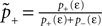 the probability that the event was a plus-event and
 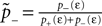 be defined analogously. Given an event (either plus or minus), the transition probability is
the probability that the event was a plus-event and be defined analogously. Given an event (either plus or minus), the transition probability is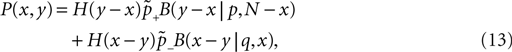
where 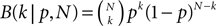 is the binomial distribution and H the Heaviside function. We are interested in the equilibrium distribution ρ(x), which must fulfill
is the binomial distribution and H the Heaviside function. We are interested in the equilibrium distribution ρ(x), which must fulfill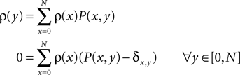
To obtain the non-trivial solution, we have to take into account the normalization condition  This results in the inhomogeneous linear system of N + 1 equations
This results in the inhomogeneous linear system of N + 1 equations
which can be solved numerically. Since the transition probability P(x, y) is a positive stochastic matrix, i.e. it fulfills P(x, y) ≥ 0 and  according to the Perron-Frobenius theorem (MacCluer, 2000
) its largest eigenvalue is 1 and the respective eigenvector ρ(x) is unique with positive entries. This guarantees a unique solution of Eq. 14 with the desired properties of a probability distribution.
according to the Perron-Frobenius theorem (MacCluer, 2000
) its largest eigenvalue is 1 and the respective eigenvector ρ(x) is unique with positive entries. This guarantees a unique solution of Eq. 14 with the desired properties of a probability distribution.
Analytic approximation of the equilibrium distribution
according to the Perron-Frobenius theorem (MacCluer, 2000
) its largest eigenvalue is 1 and the respective eigenvector ρ(x) is unique with positive entries. This guarantees a unique solution of Eq. 14 with the desired properties of a probability distribution.In order to obtain information about the equilibrium density ρ(x) we investigate its first and second moments. Suppose, x obeys the distribution ρ(x, t) at time t with a well defined first and second moment. In this case we can determine the infinitesimal time evolution of μ(t) = 〈x(t) 〉 and σ2(t) =〈(x(t) −〈x〉)2〉 for short times Δt. For the mean we obtain
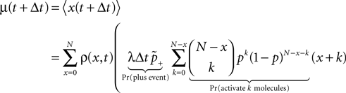
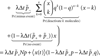
where the identity  (mean of the binomial distribution) was used. The first moment of the distribution fulfills the differential equation
(mean of the binomial distribution) was used. The first moment of the distribution fulfills the differential equation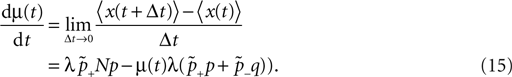
In equilibrium, the mean value is

In addition, we can calculate its temporal evolution from Eq. 15 to be

So the time scale on which the distribution approaches its equilibrium is given by
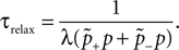
Similarly, the infinitesimal time evolution of the variance unfolds to
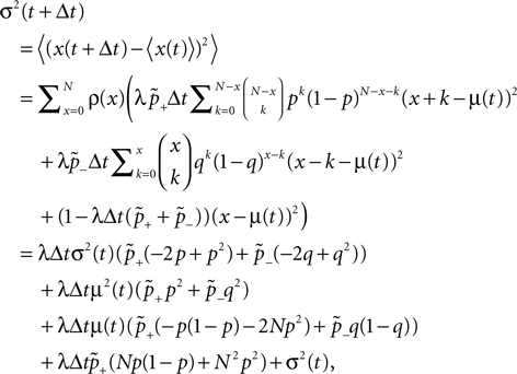
where we used  and
and  k2 = Np(1 − p) + (Np)2. We obtain the differential equation
and k2 = Np(1 − p) + (Np)2. We obtain the differential equation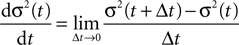
In equilibrium, we determine

Figure 11
compares the numerical solution of Eq. 14 to a Gaussian with mean μeq and standard deviation σeq, demonstrating that the Gaussian approximation is sufficient.
Mean first passage time problem for the number of
CaMKII molecules
In the model the number of active CaMKII molecules x determines whether a synapse maturates or dies. Both decisions are triggered by the crossing of different thresholds. Thus we have to calculate the mean time until x passes the threshold X for the first time. This is known as the mean first passage time problem with an absorbing boundary at x = X. Here we are interested in an approximation for the mean first passage time, or equivalently, for the threshold passing rate.
Figure 5
shows that the equilibrium distribution ρ(x) in absence of any absorbing boundary is well described by a Gaussian distribution. This observation suggests a mapping of the discrete first passage time problem to a continuous one with  and the corresponding replacement of the discrete probability distribution ρ by a continuous probability density function
and the corresponding replacement of the discrete probability distribution ρ by a continuous probability density function 
In the following we omit the tilde; x and ρ name the continuous variables. The time evolution of the probability density ρ(x) can be described by the Fokker–Planck equation

where S(x) denotes the probability flux operator. An explicit form can be determined under the following assumptions: (1) The process can be described as a diffusion. (2) The equilibrium distribution of the process is given by a Gaussian  where μeq and σeq are determined by Eqs. 16 and 17. The stationary probability density has to fulfill
  so from Eq. 19 it follows that S(x)ρ0(x) = S0 = const. The constant must be S0 = 0, since the probability current vanishes at
  it vanishes for all x. We intend to describe the process as a diffusion. Therefore, S should contain only first derivatives in x and the flux operator must have ρ0 as its stationary solution, leading to
where μeq and σeq are determined by Eqs. 16 and 17. The stationary probability density has to fulfill so from Eq. 19 it follows that S(x)ρ0(x) = S0 = const. The constant must be S0 = 0, since the probability current vanishes at it vanishes for all x. We intend to describe the process as a diffusion. Therefore, S should contain only first derivatives in x and the flux operator must have ρ0 as its stationary solution, leading to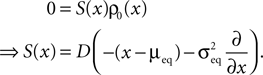
The constant D controls the time scale of the process. We determine D such that the dynamics of the diffusion process Eq. 19 matches the dynamics of our process for the first moment of ρ. In doing so, we follow Ricciardi et al. (1999) and determine the infinitesimal drift term A1(x) from the master equation of the process, which yields
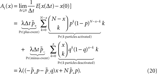
Subsequently we require A1(x) = −D(x − μeq), which fixes 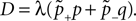
To simplify the notation, we rescale the variable  The flux operator now reads
 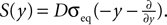 A separation ansatz for the probability density ρ(y, t) = φ(y)eηt turns the Fokker–Planck equation 19 into the corresponding eigenvalue problem
The flux operator now reads A separation ansatz for the probability density ρ(y, t) = φ(y)eηt turns the Fokker–Planck equation 19 into the corresponding eigenvalue problem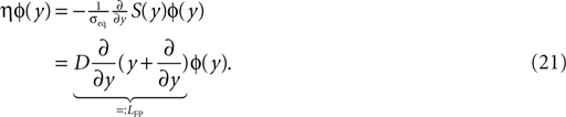
To find the eigenvalues of LFP, we follow Risken (1996) and transform Eq. 21 into a Hermitian operator, using the following transformation
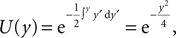
which satisfies
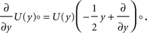
Hence the transformed operator L is
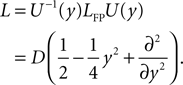
Let φ(y) be an eigenvector of LFP, then obviously ψ = U−1(y)φ(y) is an eigenvector of L with the same eigenvalue, so we have to solve
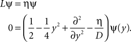
This is the differential equation of the harmonic oscillator known from quantum mechanics. The general solution of this differential equation is a linear combination of confluent hypergeometric functions (Abramowitz and Stegun, 1974
)
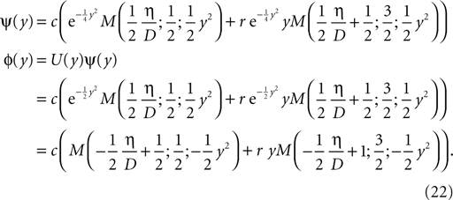
The last equality follows from M(a, b, z) = ezM(b − a, b, −z) where the constant c must be determined using the normalization condition  The boundary conditions constrain the choice of possible values for η as well as for the constants r. Without loss of generality, we assume that the threshold X has to be crossed from above (synapse pruning). The case in which the threshold represents an upper boundary (synapse maturation) can be handled analogously by interchanging the roles of plus and minus-events and the associated quantities. At the upper end
  of the interval, the probability flux has to vanish, i.e. this is a totally reflecting boundary
The boundary conditions constrain the choice of possible values for η as well as for the constants r. Without loss of generality, we assume that the threshold X has to be crossed from above (synapse pruning). The case in which the threshold represents an upper boundary (synapse maturation) can be handled analogously by interchanging the roles of plus and minus-events and the associated quantities. At the upper end of the interval, the probability flux has to vanish, i.e. this is a totally reflecting boundary
The lower end of the interval is given by the threshold X. This is an absorbing boundary, but does not require the probability density to vanish, since the rate of minus-events is limited and hence the threshold passing rate remains finite even if φ(X) > 0. The probability for the system in state x to cross the threshold X after having received a minus-event is
where the last expression is the cumulative density function of the binomial distribution. Figure 12
shows the typical steep increase of the exit probability in the vicinity of the threshold X.
The flux η through the boundary can be calculated as

The probability density can be approximated by a linear Taylor series here, since pexit(x) vanishes except in a small range near the threshold (see Figure 12
). Using the flux operator S, the flux through the boundary can be expressed as
Taken together we obtain the boundary condition
Using the explicit form of ρ given by Eq. 22, and its derivative
where we exploit the identity  the boundary condition Eq. 23 assumes the form
the boundary condition Eq. 23 assumes the form
which fixes the constant r as
Finally, we simultaneously solve Eqs. 28 and 27 for η by a simple numerical bisection method. By construction, the solutions η0 > η1>… are eigenvalues of the Fokker–Planck operator Eq. 21. Since eventually the system has to pass the threshold, there cannot be an equilibrium eigenstate with η0 = 0; all eigenstates are decaying. We are interested in the largest negative eigenvalue, which determines the slowest decaying eigenvector Eq. 22, i.e. the largest η1 < 0 which solves Eq. 21 and fulfills the boundary conditions. Being initially (t = 0) in this eigenstate, the probability of finding the system still in the interval [0, X] after time t is

where η1 is called the escape rate or the inverse mean first passage time. The eigenvector in Eq. 22 resulting from the considerations above is plotted in Figure 6
together with results of direct simulations. The decay rate expected from Eq. 29 agrees well with the simulation. In this analytical treatment we have assumed that plus and minus-events occur independently of the history of previous events with probabilities  and
and  respectively. However, this is an approximation, since plus and minus-events depend on the signal n(t), which has the time scale τnmda. Thus, given a postsynaptic spike at tpost,1 and given n(tpost,1) > Θh, a plus-event is produced. n(t) then decays exponentially with the time constant τnmda or it jumps to even higher values, if a presynaptic spike arrives. Therefore a later postsynaptic spike tpost,2 > tpost,1 definitely generates another plus-event as long as
  i.e. within a finite time window after the first event. Consequently, the probability
  for a plus-event to follow another plus-event is slightly higher than
  The same is true for minus-events. But since a neuron’s spike train exhibits refractoriness and the probability is low that the second spike occurs within the time window determined by τnmda, the correlated occurrence of plus (or analogously minus) events has only a small impact. This is verified in Figure 12
B, where the probability of k consecutive plus-events is displayed. For events caused by the spike train of an integrate and fire neuron, the curve is near its theoretically expected value
The same is true for minus-events. But since a neuron’s spike train exhibits refractoriness and the probability is low that the second spike occurs within the time window determined by τnmda, the correlated occurrence of plus (or analogously minus) events has only a small impact. This is verified in Figure 12
B, where the probability of k consecutive plus-events is displayed. For events caused by the spike train of an integrate and fire neuron, the curve is near its theoretically expected value  while for spikes with Poisson statistics, the correlated occurrence of plus-events can be explained by
  with
with 
and respectively. However, this is an approximation, since plus and minus-events depend on the signal n(t), which has the time scale τnmda. Thus, given a postsynaptic spike at tpost,1 and given n(tpost,1) > Θh, a plus-event is produced. n(t) then decays exponentially with the time constant τnmda or it jumps to even higher values, if a presynaptic spike arrives. Therefore a later postsynaptic spike tpost,2 > tpost,1 definitely generates another plus-event as long as i.e. within a finite time window after the first event. Consequently, the probability for a plus-event to follow another plus-event is slightly higher than The same is true for minus-events. But since a neuron’s spike train exhibits refractoriness and the probability is low that the second spike occurs within the time window determined by τnmda, the correlated occurrence of plus (or analogously minus) events has only a small impact. This is verified in Figure 12
B, where the probability of k consecutive plus-events is displayed. For events caused by the spike train of an integrate and fire neuron, the curve is near its theoretically expected value while for spikes with Poisson statistics, the correlated occurrence of plus-events can be explained by with Input–Output Correlation of an Integrate and Fire Neuron
Here we calculate the correlation coefficient of the incoming spike train at a given excitatory synapse and the output spike train of an integrate and fire neuron, where the correlation coefficient is defined by Eq. 10. If we have incoming Poisson spikes at a stationary rate νi, the neuron fires in a stationary fashion with rate νo as well. We can then rewrite the cross-correlation function as Cio(Δt) = νo(Δt | given an input spike at t = 0)νi and formally the correlation coefficient in Eq. 10 reads

For the particular case of Δ-shaped postsynaptic currents we find an explicit expression for Eq. 30 as follows. The membrane potential V is governed by
with reset potential Vr and spike threshold Vth. Here ti is the time of the i-th incoming event and wi its weight. For each event, the weight wi is a random variable with distribution K. This allows us to calculate Eq. 30 also for the case where a neuron receives N correlated spike trains (see section “Correlated Poisson Input”). The incoming events are assumed to be Poisson events with rate ν. Then the membrane potential is a Markov process with distribution P(V, t) which obeys the evolution equation
We closely follow the derivation of the Fokker–Planck equation for the integrate and fire neuron given by Gerstner and Kistler (2002)
, but generalize it for arbitrary weight distributions K. As we assume stationary input, we set t′ = 0 without loss of generality. For short times Δt the transition probability becomes
and the membrane potential distribution after time Δt is
Taking the limit Δt → 0 yields
A Kramers–Moyal expansion can be made under the assumption that the weight w is small and the rate ν is high. This is also known as the diffusion limit:
In the limit of small 〈w〉K only the first and the second moment of K enter the Fokker–Planck equation. This determines the drift constant μ and the diffusion constant σ2 to
In equilibrium, the firing rate νo of the neuron can be calculated by the formula (Brunel, 2000
; Brunel and Hakim, 1999
; Ricciardi, 1977
)
Finally, we employ linear response theory to calculate the input–output correlation coefficient in Eq. 30 for one particular incoming synapse in the limit of small weights w. First assume, that every event has the same weight w. Since the incoming spike rate is stationary, without loss of generality, we can assume an incoming spike to occur at time t = 0. This is a small perturbation of the membrane potential and shifts the distribution by weight w to the right, which can be taken into account in the Fokker–Planck equation 32 as
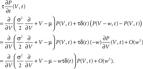
To first order in w, the incoming spike can be described as a Δ shaped perturbation of the mean input μ(t) = μ + τwΔ(t). Since the events are Poisson, their auto-correlation is flat, thus in the instant t = 0− before the spike arrives the neuron’s membrane potential obeys the equilibrium distribution. The effect of the perturbation on the firing rate can be treated in the framework of linear response theory for small w << Vth − μ. The response of the firing rate can then reads
νo(t | input spike at t = 0) = νo + wτh(t) t ≥ 0,
where νo is the equilibrium firing rate and h(t) is the impulse response of the firing rate with respect to a Δ-shaped perturbation of the mean input. So Eq. 30 becomes

where  is the step-response of the firing rate for t → ∞ with respect to a unit-step change of the mean input. Up to linear order in w
is the step-response of the firing rate for t → ∞ with respect to a unit-step change of the mean input. Up to linear order in w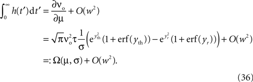
In the second step we employ Eq. 34 and in the third summarize terms by the quantity ω(μ, σ) called “dc-susceptibility” in linear response theory. Using Eq. 36 in Eq. 35 results in the desired explicit expression. A related approach can be found in De la Rocha et al. (2007)
.
Correlated poisson input
The input–output correlation coefficient can also be calculated in the case, where the neuron receives spikes from N excitatory inputs of weight w generated by a multiple-interaction-process (mip) Kuhn et al. (2003)
with mother spike rate νmother and copy probability c. In addition, the neuron receives uncorrelated excitatory and inhibitory Poisson input which we treat as a Gaussian white noise background input with mean μbg and standard deviation σbg. As in “Poission Input” we are interested in the correlation coefficient in Eq. 30 of a given input i ∈ [1,…,N] and the output spike train. A spike at time ti at input i, indicates that there is a mother-spike that was successfully copied to input i. Hence, with probability c each of the remaining N − 1 inputs also has a spike at time ti. Therefore the expectation value of the weight of the composed event is
〈w〉mip = (1 + (N − 1)c)w. For small 〈w〉mip <<Vth − μ the we can apply the framework of linear response theory as before and calculate Eq. 30 using Eqs. 36 and 35 as
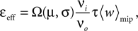
where
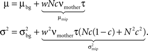
The last two equations using μmip and  result from Eq. 33.
result from Eq. 33.Algorithmic Implementation of Synapse Maturation and Synapse Death
A synapse connecting an axon of neuron i to the dendrite of neuron j is stored in a list associated with neuron i. Without loss of generality we restrict the discussion to the case of a single synapse between i and j. In a distributed simulation, each process stores only the part of the list referring to the resident target neurons (see Morrison et al., 2005
). The parameters and dynamic variables stored for each synapse j are: the synaptic weight wj, the synaptic delay  composed of the dendritic delay
  and the axonal delay
  the number xj of active CaMKII molecules, and the boolean variable maturej indicating whether the synapse is mature (True) or premature (False). Axonal delays and the NMDA receptor rise time can be taken into account as long as
  (compare Morrison et al., 2005). However, in our simulations, we assume
  for sake of simplicity. We also assume the time constant τnmda to be identical for all synapses. In this case the fraction of glutamate bound NMDA receptors n(t) as defined in Eq. 3 is the same for all axonal synapses of neuron i. In addition, each neuron stores the time told of its last spike. The spike distribution algorithm invokes the method
  the new synapse will start accessing the spike history (excluding tfirst). Analogously,
  is the latest point in the history (including tlast) considered by the synapse before dawn (see Algorithm 1).
composed of the dendritic delay and the axonal delay the number xj of active CaMKII molecules, and the boolean variable maturej indicating whether the synapse is mature (True) or premature (False). Axonal delays and the NMDA receptor rise time can be taken into account as long as (compare Morrison et al., 2005). However, in our simulations, we assume for sake of simplicity. We also assume the time constant τnmda to be identical for all synapses. In this case the fraction of glutamate bound NMDA receptors n(t) as defined in Eq. 3 is the same for all axonal synapses of neuron i. In addition, each neuron stores the time told of its last spike. The spike distribution algorithm invokes the method spike(t) (see Algorithm 1) for each spike t of the presynaptic neuron i. It propagates the dynamics of each synapse in the local target list. Here we use the function T(x, n′) (see Algorithm 2) as an abbreviation for the transitions of x due to the number n′ = n(tpost) of glutamate bound NMDA receptors as defined in the section “A Counter for Correlated Events”. To evolve the synaptic dynamics, we need the spike history of the postsynaptic neuron. Here we closely follow Morrison et al. (2007) and use the same definition of update_register(t) and get_history(t1, t2). An extension, however, is necessary, because in the presence of structural plasticity the number of incoming connections of a neuron may change over time: The access counter counterSP of each entry in the spike register has to be adapted whenever a synapse is created or dies. We define the method start_recording(tfirst) (see Algorithm 3) called on the postsynaptic neuron when a new synapse is created. The argument is the earliest the new synapse will start accessing the spike history (excluding tfirst). Analogously, stop_recording(tlast) is called when a synapse dies (see Algorithm 4). Its argument is the latest point in the history (including tlast) considered by the synapse before dawn (see Algorithm 1).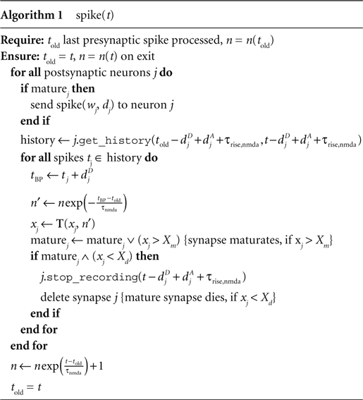
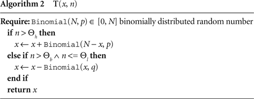
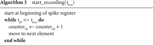
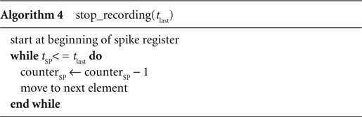
The authors declare that the research was conducted in the absence of any commercial or financial relationships that could be construed as a potential conflict of interest.
Many thanks to Birgit Kriener for very helpful discussions and to Tom Tetzlaff for comments on an earlier version of the manuscript. Ursula Körner and Andreas Knoblauch contributed essential inspiring ideas in the initial phase of the project. The implementation of the synapse model is the result of constructive discussions with the NEST initiative (www.nest-initiative.org). Partially funded by DIP F1.2, BMBF Grant 01GQ0420 to the Bernstein Center for Computational Neuroscience Freiburg, and EU Grant 15879 (FACETS), and “The Next-Generation Integrated Simulation of Living Matter” project, part of the Development and Use of the Next-Generation Supercomputer Project of the Ministry of Education, Culture, Sports, Science and Technology (MEXT) of Japan.