Neural Network Reconstruction of Plasma Space-Time

1 Introduction

Machine learning techniques for space science have grown popular in recent years, with diverse applications across the coupled Sun-Earth system. These include coronal holes (Bloch et al., 2020; Illarionov et al., 2020), solar flare forecasting (Li X. et al., 2020; Wang X. et al., 2020), solar wind prediction (Upendran et al., 2020), and space weather forecasting (Camporeale (2019) and references), among other applications. However, most of these applications use general neural network architectures, such as convolutional neural networks, which utilize large amounts of observed data for training and discovery. Although solar-disk based missions like the Solar Dynamics Observatory (Pesnell et al., 2012) are able to provide this abundance of data, other spacecraft missions (especially in planetary magnetospheres) do not have such an abundance. Indeed, magnetospheric space-based missions suffer from a sparsity problem: the amount of information they are able to measure is very tiny relative to the full scale of information present within the global system.

The usual method of “filling in the blank” for missing magnetospheric information is to perform computer simulations. If we wish to provide global context, we use large-scale, computationally-intensive global magnetohydrodyamic simulations of the magnetosphere (e.g., SWMF (Tóth et al., 2005), GAMERA (Zhang et al., 2019), OpenGCCM (Raeder et al., 2001), Gkeyll (Dong et al., 2019)). These simulations are typically initialized with solar wind conditions closest to the time of interest, and then compared directly with the spacecraft observations after run completion. Global simulations, however, are not sophisticated enough to assimilate spacecraft observations and determine the most likely magnetosphere dynamics which produced these observations. Unfortunately, it is often too computationally expensive to run multiple iterations in order to best fit the data, especially for more advanced simulations which extend beyond ideal MHD.

There have recently been great strides in using data-mining methods for this type of reconstruction. Sitnov et al. (2021) fuse nearest-neighbor regression of historical data with global magnetic field models in order to reconstruct the full magnetospheric magnetic field surrounding a particular event. However, their estimates for the plasma dynamics or the magnetic field evolution of the system are based on previous observations, and not do necessarily provide the actual time evolution of the system. Another example of combining data-mining and dynamic modeling is Chu et al. (2017), who present a neural-network-based dynamic electron density model derived from data across multiple space missions within the inner magnetosphere. This model is able to reproduce key features of plasmaspheric evolution during the erosion and refilling cycle, but it is limited to electron density.

We need a method which simultaneously provides an accurate fit to observed data but also provides a full, precise reconstruction of plasma states. We want to fully understand how events arise and will proceed within the temporal evolution of the magnetosphere. In order words, we need to be able to reconstruct the full picture surrounding spacecraft measurements, in both space and time.

In this paper, we explore the use of Physics-Informed Neural Networks (PINNs) for reconstructing information from simulated spacecraft measurements within one-dimensional hydrodynamic (HD) and magnetohydrodynamic (MHD) benchmark problems. Recently, there has been much interest in the literature about using multi-layer perceptron networks as a mesh-free method to solve partial differential equations (PDEs) at given time snapshots, akin to a least-squares finite element method. These results (e.g., Sirignano and Spiliopoulos (2018); Raissi et al. (2019); Michoski et al. (2020); Wang S. et al. (2020); Li Z. et al. (2020)) demonstrate the remarkable potential of utilizing PINNs to determine the solution to a PDE at an arbitrary time t given an initial (t = 0) and boundary conditions. The PINNs are able to incorporate the PDE behavior into their loss function, and train the model such that the output is constrained to follow this equation-defined behavior. Indeed, some authors have even begun to explore how PINNs can supplement rather than replace traditional linear solvers (Markidis, 2021). While this is a great success, much is still unknown about how well this framework scales up to more complicated situations, especially from scalar functions (like Burgers’ equation) to vector conservation laws (like the system of MHD equations). This is especially important in the context of spacecraft data reconstruction, which are often interpreted using some variety of MHD. We would eventually like to know whether or not it is possible to use one-dimensional plasma data to precisely reconstruct two- or even three-dimensional structures and environments. Although it is reasonable to assume that 1D spatio-temporal data can be used to reconstruct a 2D (1 space + 1 time) domain, it is unknown how well 1D data can apply to 3- or even 4D space-time domains.

Here, we begin this investigation by adapting a PINN model to our hypothetical (M)HD spacecraft scenario. Instead of specifying the solution at the edges of the space-time domain, we sample linear trajectories of data throughout the full domain. The observations provide a data matrix $\bar{D}=\left[{\mathbf{U}}_1,{\mathbf{U}}_2,\dots ,{\mathbf{U}}_n\right]$ for (M)HD state variables U at each sampled point (x_n, t_n) within the space-time domain. $\bar{D}$ provides the boundary constraint for our PINN, while we constrain the output via a loss-function which incorporates the (M)HD equations. The resulting solutions are then consistent with both the (M)HD equations and the spacecraft data. We note that we are not attempting to solve the underlying (M)HD equations in the same manner as more traditional computer simulations; instead, we are adapting PINN-based PDE solver techniques to our reconstructions. Similar physics-based reconstruction efforts (not using PINNs) have been applied for flux ropes and flux transfer events (Slavin et al., 2003; Sonnerup et al., 2004; DiBraccio et al., 2015), magnetopause structures (Hasegawa et al., 2006; Chen and Hau, 2018) and reconnection (Teh and Ã-. Sonnerup, 2008), and coronal mass ejections (Nieves-Chinchilla et al., 2018).

The paper is presented as follows: Section 2 provides an overview of the PINN reconstruction method, including the architecture (Figure 1) and loss function composition; Sections 3.1–3.3 detail our experience and results with the (M)HD reconstruction; and we provide a brief discussion about extension to multiple dimensions in Section 4.

FIGURE 1

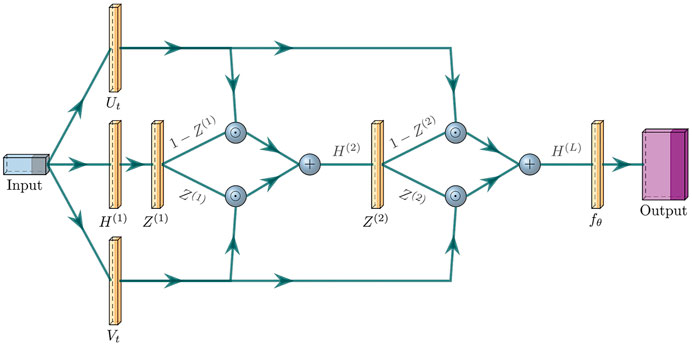
FIGURE 1. Cartoon of PINN transformer architecture described in Eqs. 5–9 for an example two-layer network (L = 2), going left to right. The yellow boxes denote fully-connected linear layers with trainable tanh activation functions. The blue spheres denote elementwise operations (ʘ and +) on their inputs.

2 Neural Network Reconstruction Method

Following Raissi et al. (2019), we create a physics-informed neural network (PINN) in order to find a solution U_net (θ; x, t) which follows both a physical constraint

$f_{net}≔\frac{\partial {\mathbf{U}}_{net}}{\partial t}+\frac{\partial F({\mathbf{U}}_{net})}{\partial x}=0(1)$

and a boundary data constraint

${\mathbf{U}}_{net}(x_i,t_i)=\mathbf{U}(x_i,t_i),i=1\dots N_b(2)$

for N_b coordinates of (x_i, t_i) in a space-time domain. In our application, U = (ρ, v_x, v_y, v_z, P, B_x, B_y, B_z) is the MHD state vector, F is the one-dimensional MHD fluxes and θ represents the parameters of the neural network U_net. The parameters θ of the PINN can be learned by minimizing the mean squared error loss MSE = L_b + λL_f, where

$L_b=\frac{1}{N_b}\sum _{i=1}^{N_b}\Vert \mathbf{U}(x_i,t_i)-{\mathbf{U}}_{net}(x_i,t_i){\Vert }^2(3)$

is the boundary data loss and

$L_f=\frac{1}{N_c}\sum _{c=1}^{N_c}\sum _{q=1}^{N_q}\Vert f_{q,net}(x_c,t_c){\Vert }^2(4)$

is the physical constraint loss. λ is the tradeoff parameter which balances the different scales between the data and physics losses. In our experiments, we found that setting λ = 1 was sufficient; however, we note that there are methods to find a more appropriate value for λ, e.g., grid search or other hyperparameter optimization techniques. We use the ADAM optimizer (Kingma and Ba, 2014) for the minimization with an initial learning rate of 1 × 10^–3 and epsilon set to 1 × 10^–4. We note that, although we did not use them in this paper, higher order optimizers, such as L-BFGS-B (Zhu et al., 1997), are likely to be necessary for more complicated reconstructions. Indeed, Markidis (2021) (using DeepXDE: (Lu et al., 2021)) demonstrate that using ADAM and then L-BFGS-B produces higher quality solutions than ADAM alone.

N_q here represents the total number of physical equations which constrain the PINN output (see Section 2.2; N_q = 9 for 1D MHD). (x_c, t_c) represent so-called “collocation points” (c.f. Raissi et al. (2019)); these points, distributed throughout the reconstruction domain, are where the physics residuals (Eq. 4) are evaluated during the training process. N_c denotes the number of collocation points used in the loss calculation during each step. For each of the individual equations, the associated loss term is created by evaluating the time and spatial derivative of each state variable with respect to the input collocation point. Minimizing the residual to zero for each of the physics loss terms is identical to having the PINN output satisfy the set of equations over the full domain. It is not enough to simply fit the data and hope the output extrapolates well to the rest of the region; forcing the learning to account for the physics residuals allows the reconstruction to capture the intended structure.

In order to appropriately cover the reconstruction domain, we generate collocation points using Latin Hypercube sampling (Iman et al., 1981); we use a implementation based on the library function pydoe2.lhs (Sjögren et al., 2018). This sampling method allows for a relatively even spread of points throughout the domain. We repeat this sampling for each training step; frequently randomizing the collocation points allows for a fuller coverage of space-time throughout training. Collocation point densities reported in this paper follow the format N², where N is the number of evenly-distributed spaces along each of the space and time dimensions; the hypercube sampling generates one randomly selected point in each of the N² boxes which make up the full sampling grid. We note that we have not attempted any sort of refinement of collocation point coverage, e.g., adding a higher density of points around steeper gradients (Lu et al., 2021).

At first, we used automatic differentiation (AD; see, e.g., history and review in Baydin et al. (2018)) to get the derivatives of the output U state vector with respect to the input (x, t) collocation points (as in Eq. 1). It is essential to get the individual derivatives since we wish for the individual equations to be satisfied independently, i.e., f_q,net = 0 for all q. However, we found that typical AD algorithms (including those in tensorflow) calculate the sum of the derivatives of the input matrix, since they use matrix-vector products. Thus, in order to get individual derivatives, we have to run the AD algorithm once per variable (8 evaluations for MHD). Otherwise, we end up with a sum of all the derivatives (i.e., ∂ρ/∂x + ∂v_x/∂x + … for MHD).

As a result, we found that it was faster to use the network output to approximate the gradient at the collocation points. To do this, we use the central difference formula ∂U/∂x ≈ [U (x + Δx) − U(x −Δx)]/2Δx (and similar for ∂U/∂t). For a given set of collocation points (x_i, t_i), we make four forward passes through the network for U(x_i ±Δx, t_i) and U(x_i, t_i ±Δt); these values are used to calculate the spatial and temporal derivatives according to the above formulae. The MHD equations (Section 2.2) also require knowing the values of U at the collocation point, so another forward pass is required to get U(x_i, t_i). These five forward passes provide all the relevant information necessary to evaluate the residuals for MHD (L_f ; Eq. 4). We arbitrarily define Δx = Δt = 0.001; there is no effect on runtime for different values since the forward pass does not depend on Δx or Δt. However, the choice must be sufficient to accurately resolve the physical structures present. Although we use numerical differentiation to calculate the MHD residuals L_f, we still use automatic differentiation to calculate the overall loss gradient with respect to the PINN parameters θ.

We note that the boundary conditions U(x_i, t_i) do not necessarily need to be defined in the traditional sense, i.e., on fixed exterior edges within the space-time domain. These would be defined at all x at t = 0 and/or for all t at particular x edges, e.g., x = x_L and x = x_R. Since we are imitating spacecraft data sampling, our boundary conditions cut across the x − t domain (e.g., black trajectory lines in Figure 2) and we do not specify edge behavior.

FIGURE 2

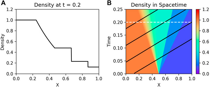
FIGURE 2. (A): Snapshot of Sod shocktube density at t = 0.2. (B): Full space-time picture of density; white line indicates t = 0.2; black lines represent trajectories of data sampling for neural network boundary fits.

2.1 Architecture

Recent studies in PINNs (e.g., Wang S. et al. (2020) and references thereof) are unclear as to the best approach for solving PDEs: most rely on the capacity of over-parameterized networks in order to reconstruct the appropriate solution of a given PDE. After experimenting with several types of fully-connected layers, including a multi-layer perceptron (Raissi et al., 2019), we found that the fully-connected transformer network presented in Wang S. et al. (2020) was the quickest to train and best reproduced the complex solutions to the benchmarks in this paper. We note that this does not necessarily mean that our choice of architecture is the best for PINNs in general. Indeed, we had difficulty adapting this network to higher dimensional reconstructions (see discussion in Section 4.1), which suggests that other kinds of architectures need to be explored in future work.

This transformer neural network architecture is designed to take advantage of residual connections within the hidden layers and multiplicative interactions between the input dimensions:

$\begin{array}{ll}\hfill U_t=& \varphi (X{W}^1+B^1);V_t=\varphi (X{W}^2+B^2)\hfill \end{array}(5)$

$\begin{array}{ll}\hfill H^{(1)}& =\varphi (X{W}^{z,1}+B^{z,1})\hfill \end{array}(6)$

$\begin{array}{ll}\hfill Z^k& =\varphi (H^k{W}^{z,k}+B^{z,k})\hfill \end{array}(7)$

$\begin{array}{ll}\hfill H^{k+1}& =(1-Z^k)ʘ{\mathit{U}}_t+Z^kʘV_t\hfill \end{array}(8)$

$\begin{array}{ll}\hfill f_{\theta }(X)& =H^{L+1}W+B,\hfill \end{array}(9)$

where k = 1 … L is the nth layer of the network, L is the number of layers, X is the (n, d) input matrix of data points, ϕ is the activation function, W and B are the weights and biases for each layer, and ʘ denotes element-wise multiplication. The input array X is an array of positions (x,t) in space-time and the output is the plasma state vector U = (ρ, v_x, v_y, v_z, P, B_x, B_y, B_z). For the space-time reconstructions in this paper, d = 2.

Although Wang et al. (2020a) used fixed hyperbolic tangent (tanh) activation functions, we found that using trainable tanh functions (e.g., Chen and Chang (1996); Jagtap et al. (2020)) delivered a more accurate reconstruction, i.e.,:

$\varphi (x)=\tanh \beta x(10)$

with β being an additional trainable parameter within each node of a hidden layer. We do not believe there is anything special about the trainable tanh functions that make it well suited for our particular class of problems; the added parameters simply allow for a greater flexibility in representing the final solution. We note that Markidis (2021) found that trainable sigmoid activation functions may work better for discontinuous source terms than trainable tanh activation functions. In general, we found that using these trainable activation functions reduced the number of steps needed for training. We refer the reader to, e.g., Apicella et al. (2020) for a survey on trainable activation functions.

Finally, our implementation environment was run on a Dell Latitude E7450 with a Intel Core i7-5600 CPU @ 2.6 GHz using Windows Subsystem for Linux. We used the tensorflow library v. 2.3.1 (Abadi et al., 2015) and python version 3.6.9. We note that the default variable dtype in tensorflow is float64, but we set the dtype in our program to float32.

Tensorflow allows GPU acceleration, but we did not experiment with this. The anticipated speedup of using a GPU would be at least 3-6x, depending on the type of GPU used.

2.2 Loss Function From Physics Constraints

We use the one-dimensional MHD equations in the derivation of our PINN physical constraint loss (Eq. 4). We use the primitive formulation along x assuming ∂/∂y = ∂/∂z = 0:

$\begin{array}{l}\hfill \frac{\partial \rho }{\partial t}+v_x\frac{\partial \rho }{\partial x}+\rho \frac{\partial v_x}{\partial x}=0\end{array}(11)$

$\begin{array}{l}\hfill \rho \frac{\partial v_x}{\partial t}+\rho v_x\frac{\partial v_x}{\partial x}+\frac{\partial P}{\partial x}+B_y\frac{\partial B_y}{\partial x}+Bz\frac{\partial B_z}{\partial x}-\rho \nu \frac{{\partial }^2{v}_x}{\partial x^2}=0\end{array}(12)$

$\begin{array}{l}\hfill \rho \frac{\partial v_y}{\partial t}+\rho v_x\frac{\partial v_y}{\partial x}-B_x\frac{\partial B_y}{\partial x}=0\end{array}(13)$

$\begin{array}{l}\hfill \rho \frac{\partial v_z}{\partial t}+\rho v_x\frac{\partial v_z}{\partial x}-B_x\frac{\partial B_z}{\partial x}=0\end{array}(14)$

$\begin{array}{l}\hfill \frac{\partial P}{\partial t}+\gamma P\frac{\partial v_x}{\partial x}+v_x\frac{\partial P}{\partial x}=0\end{array}(15)$

$\begin{array}{l}\hfill \frac{\partial B_x}{\partial t}=0\end{array}(16)$

$\begin{array}{l}\hfill \frac{\partial B_y}{\partial t}+v_x\frac{\partial B_y}{\partial x}+B_y\frac{\partial v_x}{\partial x}-B_x\frac{\partial v_y}{\partial x}=0\end{array}(17)$

$\begin{array}{l}\hfill \frac{\partial B_z}{\partial t}+v_x\frac{\partial B_z}{\partial x}+B_z\frac{\partial v_x}{\partial x}-B_x\frac{\partial v_z}{\partial x}=0,\end{array}(18)$

where we have simplified whenever possible using the 1D divergence constraint $\frac{\partial B_x}{\partial x}=0$. Each of these Eqs. 11–18 as well as the divergence constraint constitutes one term in the loss function (N_q = 9). Following Michoski et al. (2020), we add a viscosity term (ν) to the v_x equation in order to ease issues with reconstructing shock fronts and discontinuities. We generally use ν = 0.005, unless otherwise stated.

We have used the primitive variables here as opposed to the conservative variables (momentum and energy); this allows the PINN to avoid potential issues with calculating negative pressures from a conserved energy variable.

Each of the individual Eqs. 11–18 as well as the divergence constraint contributes a term to the overall loss function (Eq. 4). Since these equations are written in conservative form, we can simply calculate the time and space derivatives and sum them, e.g., for density:

$f_{1,net}≔\frac{\partial {\rho }_{net}}{\partial t}+v_{x,net}\frac{\partial {\rho }_{net}}{\partial x}+{\rho }_{net}\frac{\partial v_{x,net}}{\partial x}(19)$

where ρ_net and v_x,net are taken from the PINN-generated output vector U_net, and the derivatives are calculated numerically (as explained in Section 2).

Similarly, the hydrodynamic equation loss function is derived by setting B = 0 and removing the magnetic-related terms from the neural network output and loss function. For our hydrodynamic test problem (Section 3.1), we also ignore the v_y and v_z terms, yielding a loss function comprising of three equations (ρ, v_x, P).

3 Results

3.1 Sod Shock Tube

The Sod shock tube (Sod, 1978) is a well-known one-dimensional hydrodynamic benchmark, the solution of which comprises both shock and rarefaction waves. As such, it is an excellent problem to test the neural network reconstruction of hydrodynamic structures and waves. For the base simulation, we use a pre-existing GPU simulation code designed for solving MHD equations (Bard and Dorelli, 2014, Bard and Dorelli, 2018) and set up the Sod problem as follows:

$\begin{array}{l}\hfill {\rho }_L=1.0;{\rho }_R=0.125\\ \hfill v_L=v_R=0.0\\ \hfill P_L=1.0;P_R=0.1,\end{array}$

with a grid 0 < x < 1 and a resolution Δx = 1/8,192. The L-state was defined on 0 < x < 0.5; the R state covered 0.5 ≤ x < 1. The simulation was run until t = 0.25t₀, writing output every Δt = 0.001t₀; this provided a base space-time grid of 8,192 × 250 points, each with a state vector U_euler = (ρ, v, P), for comparison with the final neural network output.

Figure 2 illustrates the overall space-time structure for the density with a sample cut showing a 1D structure snapshot. Data was sampled along four parallel trajectories (black lines in Figure 2) and fed into the PINN as a boundary condition. Each trajectory consisted of 75 points, meaning that the boundary condition provided 300 measurements compared to the more than 2.04 million points within the overall space-time simulation grid that we saved to file.

We note that the base simulation did not need to be so highly spatially resolved; however, we did not save all of the time snapshots required to progress the simulation to t = 0.25. If we had saved the output from every time step, the full space-time dimensions would have roughly been 8,192 × 11,800 (Δt ≈ 2.12 × 10^–5 as per the CFL wave stability condition). Even a more modestly resolved simulation, e.g., nx = 512 (Δt ≈ 3.4 × 10^–4) would have full space-time dimensions of roughly 512 × 740, or about 380,000 points. Thus, the 300 points comprising the PINN boundary conditions is rather sparse compared to the overall amount of information contained within the full simulation domain. Even the collocation points, although more densely sampled, are still relatively sparse. The maximum number we reach for the Sod reconstruction is 85² = 7,225 points; the average spatial resolution between collocation points then is Δx ≈ 1/85 and the average time resolution is Δt ≈ 0.25/85 ≈ 2.9 × 10^–3.

There is no special reason for the trajectories to be parallel. We chose these to emulate the near-parallel spacecraft trajectories of constellation missions within local environments (e.g., the Magnetosphere Multiscale Mission (Burch et al., 2016) or a potential Geospace Dynamics Constellation mission (Jaynes et al., 2019)). Generally, when spacecraft measure plasma structures, it is usually the plasma that is moving much faster than the spacecraft in a solar or geospace frame of reference. Assuming a fixed plasma velocity, it is possible to translate to the plasma frame of reference; the spacecraft motions within this frame will appear as straight lines (e.g., Sonnerup et al. (2004)). We note that any contiguous (or non-contiguous) sample of data points should work with the PINN reconstruction. (See Section 3.2 for an example with non-parallel trajectories.).

More information via additional trajectories could also be provided to ensure a stronger reconstruction fit. However, our goal was to try to reproduce the simulation space-time given sparse data.

The PINN was initialized with 4 layers of 16 nodes each, following the architecture presented in Section 2.1. After some experimentation with training methodologies, we found that a learning rate schedule (e.g., Bottou (2010); Bengio (2012)) and randomization of collocation points worked very well. We first increased the density of collocation points and then decreased the learning rate upon reaching a maximum number of collocation points. We started with (N = 20)² collocation points as a “warm-up” period for the network to start fitting the boundary data, and then increased the collocation point density to (N + 5)² every 22,500 training epochs to a maximum of 85² points. When the maximum was reached, we decreased the learning rate by a factor of 2/3 until it fell below 4 × 10^–4 (from a start of 1 × 10^–3). Finally, we randomly generated a new sample of N² collocation points after each training step. After following this training schedule, the program terminates. The final training epoch count was about 280,000, taking about 3 h to run on our CPU. We could continue training by increasing the collocation point density; however, this would require a more significant time investment.

We note that the stochastic nature of neural network training means that no two PINNs will be the same, even if trained with the same loss function on the same boundary data. Despite this, we find that PINNs with the same architecture and training schedule will generally cluster around the same final reconstruction accuracy.

We plot the PINN relative error ‖(ρ_net − ρ)/ρ‖ in Figure 3. We note that the regions near the boundary trajectories are fit well, though the PINN struggles with discontinuities and shocks. Indeed, the highest error within the reconstructed regions is found immediately around the shock waves (Figure 3). Although the original MHD simulation does not have a viscosity term, adding ν to the shock parallel velocity equation (here v_x; Eq. 12) improves the fit around these abrupt gradients (corroborating Michoski et al. (2020)). This is illustrated in Figure 4; the viscosity term allows the PINN to more smoothly trace the discontinuities. This does add an artificial shock thickness in the reconstruction (lower left plot of Figure 5); this is the chief cause of the relative errors surrounding the shocks (Figure 3).

FIGURE 3

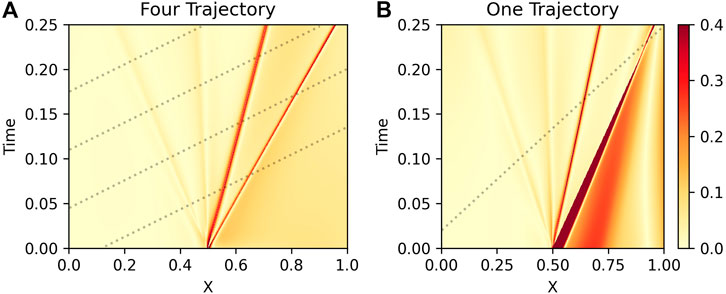
FIGURE 3. (A): Density Relative Error ‖(ρ_net − ρ)/ρ‖ for a PINN trained with four sampled trajectories (dotted lines) on the Sod shock tube. The greatest error is along the shock wave (second from right); the PINN does not handle abrupt gradients well. (B): Same, but for case of a PINN trained on one sampled trajectory. The PINN struggles to recover the solution further away from the boundary data.

FIGURE 4

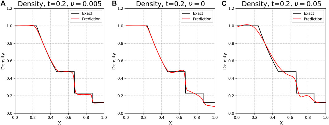
FIGURE 4. Comparison of exact values with PINN-generated predictions for ρ at t = 0.2, for different values of the viscosity term. (A): The default setting ν = 0.005. (B, C): Same, for ν = 0, 0.05. Adding a viscosity term helps the PINN generate a better fit than without, though adding too much viscosity leads to very diffusive discontinuities and a poorer fit. Without the viscosity term, the PINN struggles to resolve the shock discontinuities. All PINNs in this example were trained with the same architecture and learning schedule and for the same number of epochs, using the four-spacecraft trajectory data.

FIGURE 5

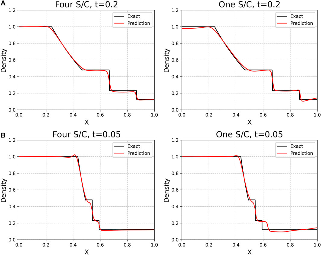
FIGURE 5. Comparison of exact simulation values with PINN-generated predictions for ρ at t = 0.2 (A) and t = 0.05 (B). The left column presents the four-spacecraft PINN fit, while the right column presents the one-spacecraft PINN fit. The PINN reconstruction tends to smooth out discontinuities and sudden gradients; this is due to adding the viscosity term (though this is still better than having no viscosity term). Additionally, the reconstruction has issues with regions further away from boundary data (lower right plot for x > 0.5; c.f. Figure 3).

Setting the viscosity too high does actively hurts the fitting in both smooth and discontinuous regions, and should be avoided. This could potentially be alleviated by, e.g., adaptive distribution of collocation points (Lu et al., 2021) by clustering them along steeper gradients (akin to adaptive mesh refinement in multi-scale plasma simulations). We note that there is no magic number for the viscosity parameter; ν = 0.005 works well here, though other similar values may give slightly better or worse results.

Since we arbitrarily chose four trajectories for the boundary data, we repeat this experiment for a single trajectory, using the same network and learning schedule as described above. In this case, the one-spacecraft PINN has a similar ability to reconstruct the domain and a similar issue with reconstruction around the shock wave. However, it has higher error in regions where it “lacks coverage”, especially in the downshock region (right portion of Figure 3; plot entitled “One Trajectory”). Interestingly, the error is lower where the single trajectory crosses the shock at a late time, but higher at an earlier time where there is less constraining information on the downshock side (lower right of Figure 5). The shock wave essentially acts as a barrier to information from upstream and makes it difficult for the PINN to constrain its reconstruction. This makes sense physically, since acoustic waves which carry information cannot travel faster than shock waves. Indeed, at t = 0.05 (Figure 5), the one-spacecraft reconstruction has difficulties with recreating the appropriate shock location and downshock state.

Ultimately, adding additional boundary data to the network training helps the PINN better constrain the solution output, especially in low-sampled areas. This raises several interesting questions: How much data is necessary for a PINN to accurately reconstruct the true environment, and how far out (in space and time) from the observed data can the PINN output be reasonably trusted? These have implications for, e.g., reconstructions of environments or magnetic structures around spacecraft observations (e.g., flux ropes (Slavin et al., 2003; Hasegawa et al., 2006; DiBraccio et al., 2015) and coronal mass ejections (Nieves-Chinchilla et al., 2018; dos Santos et al., 2020)).

Finally, we note that the PINN inference time is faster than using our GPU-based solver, though there are some caveats. For a single time snapshot, generating a full resolution 8,192 × 1 output took about 10 ms; we do not need to solve for prior times to get the solution at any given time. The full 8,192 × 250 space-time grid took about 9–10 s, compared to the original simulation time (on one NVIDIA M2090 GPU) of ≈ 40 s (including file I/O). (We note that a less resolved simulation with nx = 512 would have a runtime of several seconds.) However, this trained neural network is only effective for reconstructing this specific Sod shock tube within the given space-time extent. It is not generalizable to other shock tubes nor outside the reconstructed domain; the neural network has to be retrained for each new application.

3.2 Ryu-Jones Shock Tube

For a more complex reconstruction, we reproduce two MHD shock tubes: Ryu-Jones (Ryu and Jones, 1995) and Brio-Wu (Brio and Wu, 1988) (see Section 3.3). First, following (Ryu and Jones, 1995) (their problem 4a; henceforth referred to as RJ4a), we initialize a simple benchmark designed to test so-called “switch-on” fast shocks; the shock tube also contains several other structures. We chose the RJ4a tube as an intermediate step up to the canonical Brio-Wu shock tube (Section 3.3) since it is a less severe shock discontinuity.

The initial condition is

$\begin{array}{l}\hfill {\rho }_L=1.0;{\rho }_R=0.2\\ \hfill v_x=v_y=v_z=0\\ \hfill P_L=1.0;P_R=0.1\\ \hfill B_{y,L}=1.0;B_{y,R}=0.\\ \hfill B_x=1.;B_z=0.\end{array}$

The simulation was run until t = 0.18 with an output every Δt = 0.002; the final space-time output was represented on a 4,096 × 91 grid, each point having a full MHD state vector U = (ρ, v, P, B). As part of the spacecraft sampling, we define four non-parallel trajectories (dotted lines in Figure 6; left subfigure) and collect the plasma state data U along these tracks. Again, this is arbitrarily defined; the intent is to demonstrate that non-parallel trajectories can be used here.

FIGURE 6

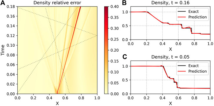
FIGURE 6. (A): Density Relative Error ‖(ρ_net − ρ)/ρ‖ for a PINN trained with four sampled trajectories (dotted lines) on the Ryu-Jones shock tube. The greatest error is along the shock wave (second from right); the PINN does not handle abrupt gradients well. (B,C): Exact (black) and NN-generated values (red) for ρ at t = 0.2 (top) and t = 0.05 (bottom). The PINN is able to reconstruct the state, but still has issues with sharp gradients.

For the MHD reconstruction, we keep the same network architecture as defined above (Section 2.1); however we adjust the number of output dimensions from 3 to 8 to reflect the full MHD state vector. Additionally, we use the full MHD loss function defined in Section 2.2. Since the reconstruction is more complex and involves more output terms and losses, the network is harder to train.

As there are roughly triple the output dimensions, we naively increase the number of nodes in each layer from 16 to 48, keeping the number of layers at 4. We also adopt a slightly different training schedule than the Sod case in Section 3.1: we start with a warm-up density of 20² collocation points for 15,000 steps, and then set the density to 30² and increase to (N + 7)² every 24,000 steps, ending at a maximum of 72² points. Upon reaching the maximum, the learning rate was decreased by a factor of 3/4 every 24,000 steps until a minimum of 2 × 10^–4 was reached. We chose 72² since the time range for the RJ4a tube is until t = 0.18 (Sod was until t = 0.25); 85²*(0.18/0.25) ≈ 72². Thus, the amount of time resolution for the collocation point distribution (Δt/N) is roughly the same for both the Rj4a and Sod reconstruction examples. The final number of steps was about 280,000, and the training time took about 8 h (alternatively: a few hours if we had used a GPU). Again, as in the Sod case, we could continue training at a higher density of collocation points at the expense of additional training time.

We are able to get similar results as the Sod shock tube: the neural network is able to reconstruct the solution space-time, albeit with issues in recreating the step discontinuity at the initial condition (t = 0) and with diffusion around the shock discontinuity. Figure 6 summarizes our results for the ρ reconstruction of the RJ4a tube, with similar results for the other reconstructed variables.

3.3 Brio-Wu Shock Tube

The final case we study, the Brio-Wu shock tube, is a well-known magnetohydrodynamic benchmark and one of the most-used MHD analogues to the Sod shock tube. It is the most difficult of our examples to train for, since it has the steepest shock discontinuity. The initial condition (Brio and Wu, 1988) is:

$\begin{array}{l}\hfill {\rho }_L=1.0;{\rho }_R=0.125\\ \hfill v_x=v_y=v_z=0\\ \hfill P_L=1.0;P_R=0.1\\ \hfill B_{y,L}=1.0;B_{y,R}=-1.0\\ \hfill B_x=0.75;B_z=0.\end{array}$

The reference dataset was created using the MHD code on a grid of 4,096 points, over a total time of t = 0.248 t₀ with an output every Δt = 0.02. This results in a space-time grid of 4,096 × 125 points. We use a similar training schedule as the RJ4a case (Section 3.2), with the exception of setting the maximum collocation point density to 85². The final number of training steps was 303,000; the training time was about 9–10 h (on CPU).

We find that the Brio-Wu shock tube is a more difficult reconstruction, especially in the shock region (Figure 7 Since we used the same architecture as the RJ4a case, part of this difficulty arises from the steeper discontinuity within the shock tube; it is harder to fit this slope with the smooth PINN output. Brief experimentation suggests that increasing the number of parameters in the network via adding more layers and/or nodes helps with a better fit; however, this also increases the training time. Alternatively, we find that increasing the viscosity to ν = 0.01 may allow the PINN to better approximate the steep discontinuity within the tube. However, as Figure 8 shows, there is not a straightforward relationship between an accurate reconstruction and choice of viscosity for each variable. Although increasing viscosity helped with the velocity reconstruction within the shock, it came at some loss of accuracy within the density reconstruction. In both cases, increasing viscosity provided a slightly less accurate reconstruction within the smooth regions. Ultimately, the key to a more accurate reconstruction with the PINN-based technique is simply to add more constraining data; the highest errors are consistently within the regions furthest away from the trajectories and on the other sides of shocks.

FIGURE 7

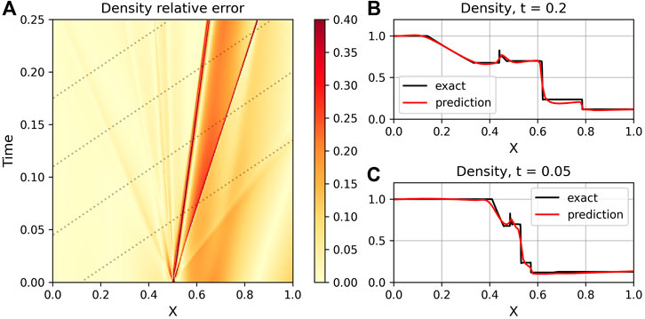
FIGURE 7. (A): Density Relative Error ‖(ρ_net − ρ)/ρ‖ for a PINN trained with four sampled trajectories (dotted lines) on the Brio-Wu shock tube. The greatest error is along the shock waves (on right side) and in the lower-right corner furthest from the sample trajectories. (B,C): Exact (black) and NN-generated values (red) for ρ at t = 0.2 (top) and t = 0.05 (bottom). The PINN is able to reconstruct the state, but still has issues around shocks.

FIGURE 8

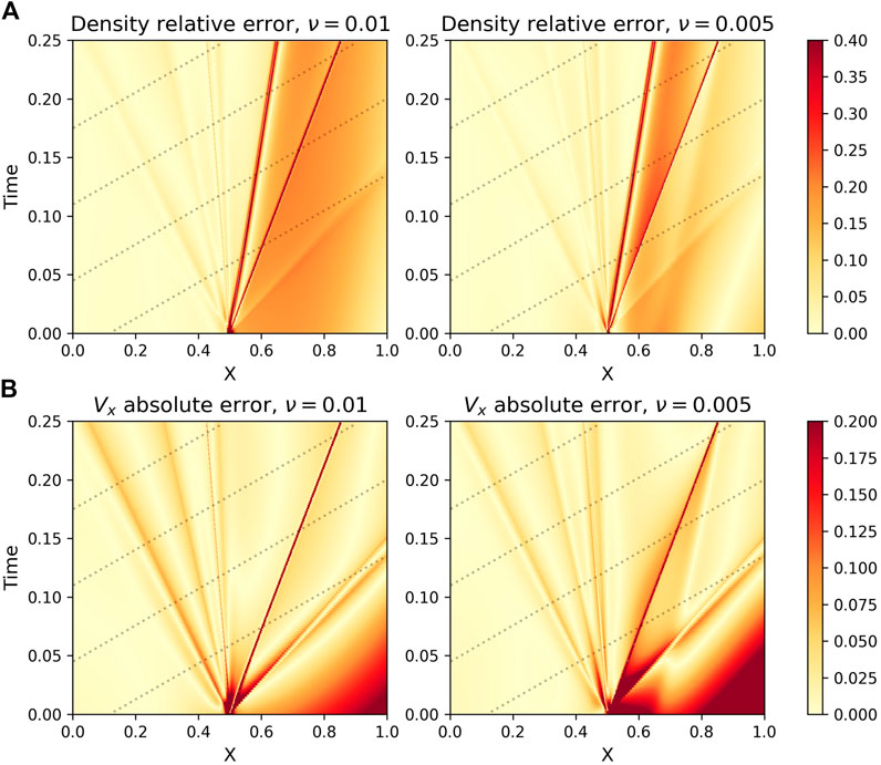
FIGURE 8. (A): Density Relative Error ‖(ρ_net − ρ)/ρ‖ for two PINNs (Left:ν = 0.01; Right:ν = 0.05) trained with four sampled trajectories (dotted lines) on the Brio-Wu shock tube. (B): Velocity Absolute Error ‖v_x,net − v_x‖ for the same PINNs as above. Both PINNs were trained with the same architecture and training schedule.

For a more direct application to spacecraft data reconstruction, we repeat the above Brio-Wu experiment with noisy trajectory data. We use the same PINN architecture and training schedule, and use ν = 0.01. The trajectory data is modified with Gaussian noise, randomly chosen from a distribution with a mean of 0 and a standard deviation of 0.1. For density and pressure, which are constrained to be positive, we set the data to a minimum of 0 where the added noise would cause negative values. Examples of noised trajectory data are shown in Figure 9.

FIGURE 9

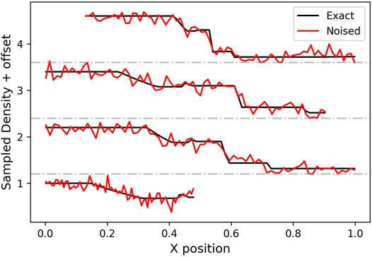
FIGURE 9. Sampled ρ data for each of the four trajectories across the Brio-Wu space-time domain, plotted as a function of X coordinate. The red line is the same data with Gaussian noise added (mean = 0, standard deviation = 0.1).

Despite the noise, the PINN is still able to reconstruct well the plasma space-time state (Figures 10–12), which bodes well for actual spacecraft data. We note that since the PINN loss function is trained on the MSE (proportional to the absolute loss), the reconstruction has a consistent level of absolute error through the space-time (except near discontinuities and domain edges). This, however, does mean that the reconstruction has similar absolute errors in both high- and low-magnitude regions, leading to a disparity in relative error between the two regions (Figures 10–12). Future work will be needed to investigate loss functions and/or training strategies such that there is a consistent level of relative error throughout the domain.

FIGURE 10

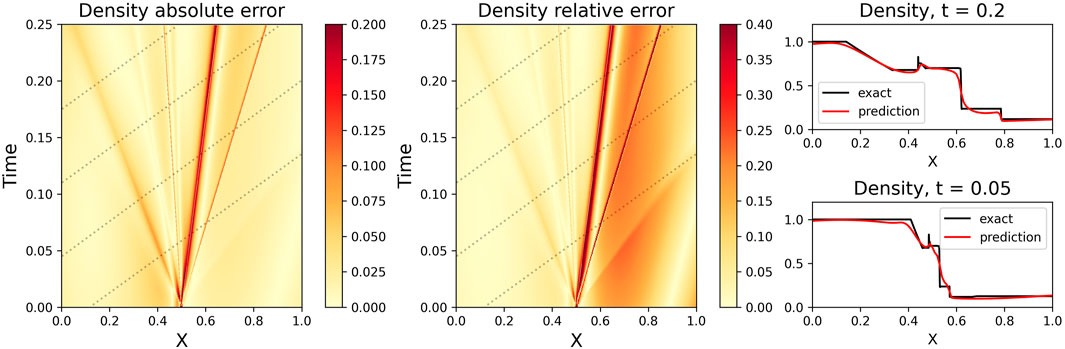
FIGURE 10. Same as Figure 7, except with ν = 0.01 and with random Gaussian noise added to the data (c.f. Figure 9). The Density absolute error ‖ρ_net − ρ‖ is also plotted. Despite the noise, the PINN obtains a similar reconstruction as the noiseless state, with similar issues around shocks and further from the constraining data. Although the relative error is higher on the right side of the shock, the absolute error is of the same order on either side of the reconstruction. Since the PINN loss function uses MSE, it minimizes the absolute error without regard to the relative magnitude difference of the actual value.

FIGURE 11

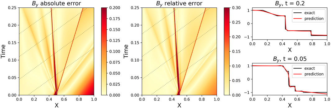
FIGURE 11. Same as Figure 10, except plotting both the B_y absolute error ‖B_y,net − B_y‖ and the B_y relative error ‖(B_y,net − B_y)/B_y‖, and B_y at selected times. Random Gaussian noise (c.f. Figure 9) has been added to the data.

FIGURE 12

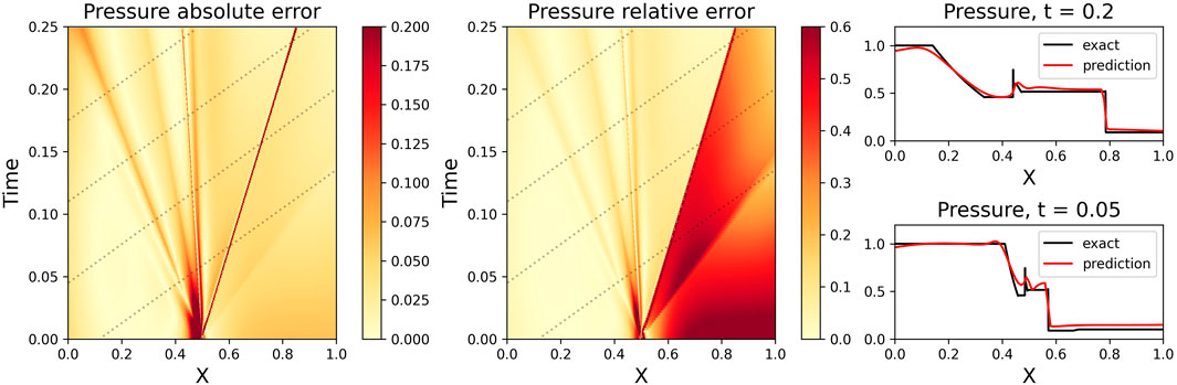
FIGURE 12. Same as Figure 11, except for Pressure. Random Gaussian noise (c.f. Figure 9) has been added to the data.

4 Discussion and Conclusion

4.1 Extension to Higher Dimensions

With the success of reconstructing the 1D MHD Brio-Wu test problem, we attempted to extend this method to a two-dimensional test problem. It was very easy to modify our architecture for 2D space + 1D time reconstruction: simply extend the loss function to include additional derivatives and modify the collocation point generator for three dimensions. However, we quickly found out that this training methodology did not scale well to higher dimensions.

Extending the collocation point strategy from 2 to 3 dimensions, while straightforward, meant that the computational intensity increased by many orders of magnitude. Sampling a similarly-sized space-time with the same density of points means that the total number of collocation points increases from N² to N³, where N is the number of points sampling across one particular dimension. In general, D dimensions of space-time require N^D collocation points.

Since the Brio-Wu test case ended with 85² collocation points, achieving a similar resolution in our 2D test case means we must use 85³ collocation points. If instead, we used a similar number of collocation points, we would be using ≈ 19³ collocation points. The collocation density would be reduced by a factor of about 4.5 in each dimension, and 90x overall! This is not nearly enough to get a reasonable solution in 3D space-time. Essentially, in the absence of ever-faster computer processing (e.g., multiple GPUs), the trade-off is between a significant increase in reconstruction time or a large decrease in reconstruction accuracy. Furthermore, the amount of reconstruction required increases with additional dimensions; more specifically, the relative amount of input data significantly decreases compared to the overall space-time information. We could add more sampled data from the baseline simulation to help with this issue, but, in the real magnetosphere, we often do not have the ability to add more spacecraft data within the local environment.

Ultimately, although this collocation point strategy does not scale well in training, we believe that it will still work to reconstruct multiple spatial and time dimensions (provided a large enough computational capability and sufficient boundary information). However, since networks are only trained on a single event, we are skeptical that reusing trained networks for different kinds of events will be viable. This transformer network + collocation point approach does not seem to be the best option for replacing global simulations in extracting the full temporal and spatial global environment information from satellite observations. But, this technique may work well for reconstructing simpler cases at smaller scales, e.g., equilibrium or force-free flux ropes (Slavin et al., 2003; DiBraccio et al., 2015), current sheets (Hasegawa et al., 2019), magnetopause structures (Hasegawa et al., 2006; Chen and Hau, 2018), coronal mass ejections (e.g., dos Santos et al. (2020)), or other geospace magnetic structures.

4.2 Conclusion

We have presented a physics-informed, fully-connected transformer neural network based on Raissi et al. (2019); Wang S. et al. (2020) which is capable of reconstructing (M)HD space-time plasma states from simulated spacecraft measurements in one spatial dimension. This reconstruction works well even in the presence of noise. We concur with Michoski et al. (2020) that the PINN has difficulties around discontinuities, like shocks, and that adding a viscosity term helps with the reconstruction in these regions. Although the PINN output has a generally consistent absolute error, this leads to a disparity of relative error between domains of high and low magnitudes.

The combination of a transformer-based architecture and the collocation point method works well, but it does take more time to train the network to find the reconstructed solution than to simulate the solution in the first place. We conclude that future implementations of PINN-based reconstruction techniques must take full advantage of GPUs for speedup. Additionally, higher-order loss optimizers, like L-BFGS-B, should be utilized when possible, as they increase training accuracy (Markidis, 2021). Ultimately, alternative network architectures and training strategies need to be explored to maximize reconstruction efficiency and accuracy.

We believe that PINN reconstruction will work in general for spacecraft data; however, there are still some significant questions concerning uncertainty. We were able to iterate the architecture and the training process over the course of this work, but this was because we had known underlying data. How can we do this in the presence of an unknown baseline? How do we quantify the uncertainty of the reconstruction, especially in space environments and with noisy data?

Other interesting questions to explore are how much data is necessary for a reliable reconstruction, and how much error due to noise or instrument mis-calibration can be tolerated? Will one-dimensional spatio-temporal data samples provide sufficient information for the reconstruction of a three-spatial + one-time dimensional reconstruction?

How far out from the spacecraft sampling are we able to go before the PINN starts making up realities that still fit the underlying physics equation? This is an issue, especially in regions where shocks are common. Unless the data transects the discontinuity, the PINN does not have the information to reconstruct the other side of the shock. We see this in the scenarios of Figures 3, 8, where the reconstruction suffers near the shock discontinuity. This can be alleviated by adding more constraining data, though this is not always possible. Future investigations on PINN error and convergence for solutions of PDEs are needed. Mishra and Molinaro (2020) is one such example: they have looked at PINN errors for solutions to several problems, including the heat, wave, and Stokes equations.

Finally, with the advent of constellation spacecraft missions like MMS (Burch et al., 2016) and GDC (Jaynes et al., 2019), we can use these multi-point spacecraft observations for more detailed reconstructions of plasma and magnetic field structures, as some have already started doing with MHD equilibriums and current sheets (Hasegawa et al., 2006, 2019). Will PINN-based techniques be an upgrade over these methods? Indeed, Chu et al. (2017); Sitnov et al. (2021) have already started doing versions of this by combining magnetometer data across many spacecraft missions, and utilizing neural-network based methods for the analysis. Fusing data with advanced models will be an exciting avenue of research for space physics in the next decade.

Data Availability Statement

The datasets presented in this study can be found in online repositories. The names of the repository/repositories and accession number(s) can be found below: The datasets generated and code created for this study will be made publicly available after acceptance of this paper as part of the NASA Open Source Code Base at code.nasa.gov. The author may be emailed for the code/data prior to final approval for public release.

Author Contributions

CB wrote the article, developed the code and ran experiments. JD secured funding, provided the computer cluster, helped edit the article, and provided feedback on method development.

Funding

The authors acknowledge support from an internal NASA Science Task Group development grant from the GSFC Sciences and Exploration Directorate, and the GSFC Heliophysics Internal Scientist Funding Model (ISFM).

Conflict of Interest

The authors declare that the research was conducted in the absence of any commercial or financial relationships that could be construed as a potential conflict of interest.

Publisher’s Note

All claims expressed in this article are solely those of the authors and do not necessarily represent those of their affiliated organizations, or those of the publisher, the editors and the reviewers. Any product that may be evaluated in this article, or claim that may be made by its manufacturer, is not guaranteed or endorsed by the publisher.

Acknowledgments

The authors thank Daniel da Silva for general discussion and feedback and the GSFC Center for HelioAnalytics for general discussion. We thank both referees for their helpful comments which improved this paper.

References

Abadi, M., Agarwal, A., Barham, P., Brevdo, E., Chen, Z., Citro, C., et al. (2015). [Dataset]. TensorFlow: Large-Scale Machine Learning on Heterogeneous Systems. Software available from tensorflow.org.

Apicella, A., Donnarumma, F., Isgrò, F., and Prevete, R. (2020). A Survey on Modern Trainable Activation Functions. arXiv e-prints. arXiv:2005.00817.

Bard, C. M., and Dorelli, J. C. (2014). A Simple GPU-Accelerated Two-Dimensional MUSCL-Hancock Solver for Ideal Magnetohydrodynamics. J. Comput. Phys. 259, 444–460. doi:10.1016/j.jcp.2013.12.006

CrossRef Full Text | Google Scholar

Bard, C., and Dorelli, J. C. (2018). On the Role of System Size in Hall MHD Magnetic Reconnection. Phys. Plasmas 25, 022103. doi:10.1063/1.5010785

CrossRef Full Text | Google Scholar

Baydin, A. G., Pearlmutter, B. A., Radul, A. A., and Siskind, J. M. (2018). Automatic Differentiation in Machine Learning: a Survey. J. Machine Learn. Res. 18, 1–43.

Google Scholar

Bengio, Y. (2012). Practical Recommendations for Gradient-Based Training of Deep Architectures. arXiv e-prints. arXiv:1206.5533.

Bloch, T., Watt, C., Owens, M., McInnes, L., and Macneil, A. R. (2020). Data-Driven Classification of Coronal Hole and Streamer Belt Solar Wind. Sol. Phys. 295, 41. doi:10.1007/s11207-020-01609-z

CrossRef Full Text | Google Scholar

Bottou, L. (2010). Large-scale Machine Learning with Stochastic Gradient Descent. In COMPSTAT. doi:10.1007/978-3-7908-2604-3_16

CrossRef Full Text | Google Scholar

Brio, M., and Wu, C. C. (1988). An Upwind Differencing Scheme for the Equations of Ideal Magnetohydrodynamics. J. Comput. Phys. 75, 400–422. doi:10.1016/0021-9991(88)90120-9

CrossRef Full Text | Google Scholar

Burch, J. L., Moore, T. E., Torbert, R. B., and Giles, B. L. (2016). Magnetospheric Multiscale Overview and Science Objectives. Magnetos. Multiscale Over. Sci. Object. 199, 5–21. doi:10.1007/s11214-015-0164-910.1007/978-94-024-0861-4_2

CrossRef Full Text | Google Scholar

Camporeale, E. (2019). The Challenge of Machine Learning in Space Weather: Nowcasting and Forecasting. Space Weather 17, 1166–1207. doi:10.1029/2018sw002061

CrossRef Full Text | Google Scholar

Chen, C.-T., and Chang, W.-D. (1996). A Feedforward Neural Network with Function Shape Autotuning. Neural Netw. 9, 627–641. doi:10.1016/0893-6080(96)00006-8

CrossRef Full Text | Google Scholar

Chen, G.-W., and Hau, L.-N. (2018). Grad-Shafranov Reconstruction of Earth's Magnetopause with Temperature Anisotropy. J. Geophys. Res. Space Phys. 123, 7358–7369. doi:10.1029/2018JA025842

CrossRef Full Text | Google Scholar

Chu, X., Bortnik, J., Li, W., Ma, Q., Denton, R., Yue, C., et al. (2017). A Neural Network Model of Three-Dimensional Dynamic Electron Density in the Inner Magnetosphere. J. Geophys. Res. (Space Phys.) 122, 9183–9197. doi:10.1002/2017JA024464

CrossRef Full Text | Google Scholar

DiBraccio, G. A., Slavin, J. A., Imber, S. M., Gershman, D. J., Raines, J. M., Jackman, C. M., et al. (2015). MESSENGER Observations of Flux Ropes in Mercury’s Magnetotail. Planet. Space Sci. 115, 77–89. doi:10.1016/j.pss.2014.12.016

CrossRef Full Text | Google Scholar

Dong, C., Wang, L., Hakim, A., Bhattacharjee, A., Slavin, J. A., DiBraccio, G. A., et al. (2019). Global Ten-Moment Multifluid Simulations of the Solar Wind Interaction with Mercury: From the Planetary Conducting Core to the Dynamic Magnetosphere. Geophys. Res. Lett. 46, 11,584–11,596. doi:10.1029/2019GL083180

CrossRef Full Text | Google Scholar

dos Santos, L. F. G., Narock, A., Nieves-Chinchilla, T., Nuñez, M., and Kirk, M. (2020). Identifying Flux Rope Signatures Using a. Deep Neural Netw. 295, 131. doi:10.1007/s11207-020-01697-x

CrossRef Full Text | Google Scholar

Hasegawa, H., Sonnerup, B. U. Ö., Owen, C. J., Klecker, B., Paschmann, G., Balogh, A., et al. (2006). The Structure of Flux Transfer Events Recovered from Cluster Data. Ann. Geophysicae 24, 603–618. doi:10.5194/angeo-24-603-2006

CrossRef Full Text | Google Scholar

Hasegawa, H., Denton, R. E., Nakamura, R., Genestreti, K. J., Nakamura, T. K. M., Hwang, K. J., et al. (2019). Reconstruction of the Electron Diffusion Region of Magnetotail Reconnection Seen by the MMS Spacecraft on 11 July 2017. J. Geophys. Res. (Space Physics) 124, 122–138. doi:10.1029/2018ja026051

CrossRef Full Text | Google Scholar

Illarionov, E., Kosovichev, A., and Tlatov, A. (2020). Machine-learning Approach to Identification of Coronal Holes in Solar Disk Images and Synoptic Maps. Astrophys. J. 903, 115. doi:10.3847/1538-4357/abb94d

CrossRef Full Text | Google Scholar

Iman, R. L., Helton, J. C., and Campbell, J. E. (1981). An Approach to Sensitivity Analysis of Computer Models: Part I—Introduction, Input Variable Selection and Preliminary Variable Assessment. J. Qual. Technol. 13, 174–183. doi:10.1080/00224065.1981.11978748

CrossRef Full Text | Google Scholar

Jagtap, A. D., Kawaguchi, K., and Karniadakis, G. E. (2020). Adaptive Activation Functions Accelerate Convergence in Deep and Physics-Informed Neural Networks. J. Comput. Phys. 404, 109136. doi:10.1016/j.jcp.2019.109136

CrossRef Full Text | Google Scholar

Jaynes, A., and Ridley, A.the GDC STDT (2019). NASA Science and Technology Definition Team for the Geospace Dynamics Constellation Final Report. Tech. Rep.

Google Scholar

Kingma, D. P., and Ba, J. (2014). Adam: A Method for Stochastic Optimization. arXiv e-prints. arXiv:1412.6980.

Li, X., Zheng, Y., Wang, X., and Wang, L. (2020a). Predicting Solar Flares Using a Novel Deep. Convolutional Neural Netw. 891, 10. doi:10.3847/1538-4357/ab6d04

CrossRef Full Text | Google Scholar

Li, Z., Kovachki, N., Azizzadenesheli, K., Liu, B., Bhattacharya, K., Stuart, A., et al. (2020b). Fourier Neural Operator for Parametric Partial Differential Equations. arXiv e-prints. arXiv:2010.08895.

Lu, L., Meng, X., Mao, Z., and Karniadakis, G. E. (2021). DeepXDE: A Deep Learning Library for Solving Differential Equations. SIAM Rev. 63, 208–228. doi:10.1137/19m1274067

CrossRef Full Text | Google Scholar

Markidis, S. (2021). The Old and the New: Can Physics-Informed Deep-Learning Replace Traditional Linear Solvers? arXiv e-prints. arXiv:2103.09655.

Michoski, C., Milosavljević, M., Oliver, T., and Hatch, D. R. (2020). Solving Differential Equations Using Deep Neural Networks. Neurocomputing 399, 193–212. doi:10.1016/j.neucom.2020.02.015

CrossRef Full Text | Google Scholar

Mishra, S., and Molinaro, R. (2020). Estimates on the Generalization Error of Physics Informed Neural Networks (PINNs) for Approximating a Class of Inverse Problems for PDEs. arXiv e-prints. arXiv:2007.01138.

Nieves-Chinchilla, T., Linton, M. G., Hidalgo, M. A., and Vourlidas, A. (2018). Elliptic-cylindrical. Anal. Flux Rope Model Magn. Clouds 861, 139. doi:10.3847/1538-4357/aac951

CrossRef Full Text | Google Scholar

Pesnell, W. D., Thompson, B. J., and Chamberlin, P. C. (2012). The Solar Dynamics Observatory (SDO). Sol. Dyn. Obs. 275, 3–15. doi:10.1007/s11207-011-9841-3

CrossRef Full Text | Google Scholar

Raeder, J., McPherron, R. L., Frank, L. A., Kokubun, S., Lu, G., Mukai, T., et al. (2001). Global Simulation of the Geospace Environment Modeling Substorm challenge Event. J. Geophys. Res. (Space Physics) 106, 381–396. doi:10.1029/2000JA000605

CrossRef Full Text | Google Scholar

Raissi, M., Perdikaris, P., and Karniadakis, G. E. (2019). Physics-informed Neural Networks: A Deep Learning Framework for Solving Forward and Inverse Problems Involving Nonlinear Partial Differential Equations. J. Comput. Phys. 378, 686–707. doi:10.1016/j.jcp.2018.10.045

CrossRef Full Text | Google Scholar

Ryu, D., and Jones, T. W. (1995). Numerical Magnetohydrodynamics in Astrophysics. Alg. Tests One-dimens. Flow 442, 228. doi:10.1086/175437

CrossRef Full Text | Google Scholar

Sirignano, J., and Spiliopoulos, K. (2018). DGM: A Deep Learning Algorithm for Solving Partial Differential Equations. J. Comput. Phys. 375, 1339–1364. doi:10.1016/j.jcp.2018.08.029

CrossRef Full Text | Google Scholar

Sitnov, M., Stephens, G., Motoba, T., and Swisdak, M. (2021). Data Mining Reconstruction of Magnetotail Reconnection and Implications for its First-Principle Modeling. Front. Phys. 9, 90. doi:10.3389/fphy.2021.644884

CrossRef Full Text | Google Scholar

Sjögren, R., Svensson, D., Lee, A. D., Baudin, M., Christopoulou, M., Collette, Y., et al. (2018). [Dataset]. Pydoe2. Available at: https://github.com/clicumu/pyDOE2 (Accessed May, 2020).

Slavin, J. A., Lepping, R. P., Gjerloev, J., Fairfield, D. H., Hesse, M., Owen, C. J., et al. (2003). Geotail Observations of Magnetic Flux Ropes in the Plasma Sheet. J. Geophys. Res. (Space Physics) 108, 1015. doi:10.1029/2002JA009557

CrossRef Full Text | Google Scholar

Sod, G. A. (1978). Review. A Survey of Several Finite Difference Methods for Systems of Nonlinear Hyperbolic Conservation Laws. J. Comput. Phys. 27, 1–31. doi:10.1016/0021-9991(78)90023-2

CrossRef Full Text | Google Scholar

Sonnerup, B. U. Ö., Hasegawa, H., and Paschmann, G. (2004). Anatomy of a Flux Transfer Event Seen by Cluster. Geophys. Res. Lett. 31, L11803. doi:10.1029/2004GL020134

CrossRef Full Text | Google Scholar

Teh, W. L., and Ã-. Sonnerup, B. U. (2008). First Results from Ideal 2-D MHD Reconstruction: Magnetopause Reconnection Event Seen by Cluster. Ann. Geophysicae 26, 2673–2684. doi:10.5194/angeo-26-2673-2008

CrossRef Full Text | Google Scholar

Tóth, G., Sokolov, I. V., Gombosi, T. I., Chesney, D. R., Clauer, C. R., de Zeeuw, D. L., et al. (2005). Space Weather Modeling Framework: A New Tool for the Space Science Community. J. Geophys. Res. (Space Phys.) 110, A12226. doi:10.1029/2005JA011126

CrossRef Full Text | Google Scholar

Upendran, V., Cheung, M. C. M., Hanasoge, S., and Krishnamurthi, G. (2020). Solar Wind Prediction Using Deep Learning. Space Weather 18, e02478. doi:10.1029/2020sw002478

CrossRef Full Text | Google Scholar

Wang, S., Teng, Y., and Perdikaris, P. (2020a). Understanding and Mitigating Gradient Pathologies in Physics-Informed Neural Networks. arXiv e-prints. arXiv:2001.04536.

Wang, X., Chen, Y., Toth, G., Manchester, W. B., Gombosi, T. I., Hero, A. O., et al. (2020b). Predicting Solar Flares with Machine Learning. Invest. Sol. Cycle Depend. 895, 3. doi:10.3847/1538-4357/ab89ac

CrossRef Full Text | Google Scholar

Zhang, B., Sorathia, K. A., Lyon, J. G., Merkin, V. G., Garretson, J. S., and Wiltberger, M. (2019). GAMERA: A Three-Dimensional Finite-Volume MHD Solver for Non-orthogonal Curvilinear Geometries. Astrophys. J. Suppl. Ser. 244, 20. doi:10.3847/1538-4365/ab3a4c

CrossRef Full Text | Google Scholar

Zhu, C., Byrd, R. H., Lu, P., and Nocedal, J. (1997). Algorithm 778: L-Bfgs-B: Fortran Subroutines for Large-Scale Bound-Constrained Optimization. ACM Trans. Math. Softw. 23, 550–560. doi:10.1145/279232.279236

CrossRef Full Text | Google Scholar