Variant Approach for Identifying Spurious Relations That Deep Learning Models Learn

A deep learning (DL) model learns a function relating a set of input variables with a set of target variables. While the representation of this function in form of the DL model often lacks interpretability, several interpretation methods exist that provide descriptions of the function (e.g., measures of feature importance). On the one hand, these descriptions may build trust in the model or reveal its limitations. On the other hand, they may lead to new scientific understanding. In any case, a description is only useful if one is able to identify if parts of it reflect spurious instead of causal relations (e.g., random associations in the training data instead of associations due to a physical process). However, this can be challenging even for experts because, in scientific tasks, causal relations between input and target variables are often unknown or extremely complex. Commonly, this challenge is addressed by training separate instances of the considered model on random samples of the training set and identifying differences between the obtained descriptions. Here, we demonstrate that this may not be sufficient and propose to additionally consider more general modifications of the prediction task. We refer to the proposed approach as variant approach and demonstrate its usefulness and its superiority over pure sampling approaches with two illustrative prediction tasks from hydrometeorology. While being conceptually simple, to our knowledge the approach has not been formalized and systematically evaluated before.

1. Introduction

A deep learning (DL) model learns a function relating a set of input variables with a set of target variables. While DL models excel in terms of predictive performance, the representation of the learned function in form of the DL model (e.g., in form of a neural network) often lacks interpretability. To address this lack of interpretability, several interpretation methods have been developed (see e.g., Gilpin et al., 2018; Montavon et al., 2018; Zhang and Zhu, 2018; Molnar, 2019; Samek et al., 2021) providing descriptions of the learned function (e.g., measures of feature importance, FI). On the one hand, such descriptions can build trust in a model (Ribeiro et al., 2016) or reveal a model's limitations. Lapuschkin et al. (2019), for example, analyzed FI scores and found that their image classifier relied on a copyright tag on horse images. Similarly, Schramowski et al. (2020) analyzed FI scores and found (and corrected) that their DL model classified sugar beet leaves as healthy or diseased while incorrectly focusing on areas outside of the leaves.

On the other hand, descriptions of the learned function can lead to new scientific understanding. Ham et al. (2019), for example, analyzed FI scores and identified a previously unreported precursor of the Central-Pacific El Ni$\widetilde{\mathrm{\text{n}}}$o type; Gagne et al. (2019) analyzed FI scores to gain a better understanding of the relations between environmental features and severe hail; McGovern et al. (2019) analyzed FI scores to gain a better understanding of the formation of tornadoes; and Toms et al. (2020) analyzed FI scores and identified regions related to the El Ni$\widetilde{\mathrm{\text{n}}}$o-Southern Oscillation (ENSO) and regions providing predictive capabilities for land surface temperatures at seasonal scales. Roscher et al. (2020) provide a general review of explainable machine learning for scientific insights in the natural sciences.

Whether descriptions of the function that a DL model learns are computed to build trust in the model, study the model's limitations, or gain new scientific understanding, it is important to identify if parts of a description reflect spurious instead of causal relations (e.g., random associations in the training data instead of associations due to a physical process). Examples for spurious relations are the above-mentioned copyright tag on horse images and the area outside of the classified sugar beet leaves. However, especially in prediction tasks involving physical, biological or chemical systems with several non-linearly interacting components, identifying spurious relations is challenging even for experts. Note that this does not only apply to the identification of spurious relations in descriptions of functions that DL models learn, but in general to the identification of spurious relations in descriptions of functions that any statistical model learns.

Commonly, this challenge is addressed by training separate instances of the considered model on random samples of the training set and aggregating or comparing the obtained descriptions. De Bin et al. (2015), for instance, compared subsampling and bootstrapping for the identification of relevant input variables in multivariable regression tasks. They applied a feature selection strategy repeatedly to samples of the original training set obtained by subsampling or bootstrapping, respectively, and identified relevant features by analyzing feature selection frequencies. As another example, Gagne et al. (2019) trained 30 instances of different statistical models on sampled training and test sets to take into account that the models' skills and the relations between input and target variables that the models learn might depend on the specific training and test set composition. Here, we propose to not only consider sampling, but also more general modifications of the original prediction task. We refer to this more general approach as variant approach. In the approach, separate instances of the considered statistical model (referred to as variant models) are trained on modified prediction tasks (referred to as variant tasks) for which it is assumed that causal relations between input and target variables either remain stable or vary in specific ways. Subsequently, the descriptions of the functions that original and variant models learn are compared and it is evaluated whether they reflect the assumed stability or specific variation, respectively, of causal relations. If this is not the case for some parts of the descriptions, these parts likely reflect spurious relations. The approach constitutes a generalization of sampling approaches in that sampling is one of many ways for modifying the original prediction task in order to obtain a variant task.

A similar concept to ours has, to the best of our knowledge, only been pursued systematically in a strict causality framework [for details on this framework see e.g., Pearl, 2009 or for a more methodological focus (Guo et al., 2020)]. Peters et al. (2016), for example, consider modifications of an original prediction task for which they require the conditional distribution $p(y|{\overrightarrow{x}}_S)$ of the target variable y given the complete set ${\overrightarrow{x}}_S$ of variables that directly cause y to remain stable. Exploiting this requirement, they aim to identify the subset S of (direct) causal predictors within all observed features. While this approach is conceptually related to the proposed variant approach, the latter does not require the strict causality framework but is applicable to any machine learning prediction task. Note that in our work the terms causal and spurious do not refer to an underlying causal graph or other concepts from the strict causality framework but should be interpreted with common sense: a pixel in an image, for instance, is causally related to the label “dog” if and only if it belongs to a dog in the image, and the value of a meteorological variable at a specific location and time is causally related to the value of a meteorological variable at another location and time if and only if one value influences the other via some physical process.

Other approaches in machine learning that consider modifications of an original prediction task predominantly aim to improve the predictive performance of a statistical model rather than to analyze the relations between input and target variables. Transfer learning (Pan and Yang, 2010), for instance, aims to extract knowledge from one or more source tasks to apply it to a target task, e.g., training a neural network first on a similar task before fine-tuning the weights on the target task. Adversarial training, as another example, optimizes the loss over a set of perturbations of the input (Goodfellow et al., 2015; Sinha et al., 2018) to become less susceptible to adversarial attacks (Szegedy et al., 2014), imperceptible changes to the input that can change the model's prediction. Traditional importance weighting (Shimodaira, 2000) or more recent methods (Lakkaraju et al., 2020), as further examples, shift the input distribution in order to perform better on a known or unknown test distribution.

In this work, we demonstrate the proposed variant approach with two illustrative prediction tasks from hydrometeorology. First, we predict the occurrence of rain at a target location, given geopotential fields at different pressure levels in a surrounding region. Second, we predict the water level at a location in a river, given the water level upstream and downstream 48 h earlier. As statistical models, we consider linear models and neural networks. After training a model on one of these tasks, we apply an interpretation method to obtain a description of the learned function. This description indicates the average importance of the different input locations for the predictions of the model. To identify if this importance reflects spurious instead of causal relations between input and target variables, we apply the proposed variant approach.

The article is structured as follows: in section 2, we formalize the variant approach and define the two prediction tasks and variants thereof that illustrate the approach. Further, we introduce the statistical models and interpretation methods used in this work. Subsequently, we present and discuss the results obtained when training the statistical models on the considered prediction tasks and applying the variant approach. In section 4, we summarize our main findings and discuss perspectives for future research and applications of the variant approach.

2. Materials and Methods

2.1. Variant Approach

During the training phase, a statistical model learns a function f:ℝⁿ → ℝ^k relating an input space X ⊆ ℝⁿ with a target space Y ⊆ ℝ^k given a training set $T={\left\{(\overrightarrow{x_i},\overrightarrow{y_i})\right\}}_{i=1}^N$ with $\overrightarrow{x_i}\in X$, $\overrightarrow{y_i}\in Y$. As the representation of f in form of the statistical model (e.g., in form of a neural network) often lacks interpretability, several interpretation methods have been developed (see e.g., Gilpin et al., 2018; Montavon et al., 2018; Zhang and Zhu, 2018; Molnar, 2019; Samek et al., 2021). Most of these methods yield vector-valued descriptions $\overrightarrow{d}\in {ℝ}^d$ of f (e.g., measures of feature importance). These descriptions can be global or local, in the latter case not only depending on f but on a subset X_d⊂X as well. An example of a global description are the weights of a linear regression model. An example of a local description $\overrightarrow{d}(\overrightarrow{x})$ is the gradient of a neural network evaluated at a location $\overrightarrow{x}\in X$.

A description $\overrightarrow{d}$ reflects the relations between input and target variables that the statistical model learned. Whether the user aims to use $\overrightarrow{d}$ to build trust in the model, reveal the model's limitations, or gain new scientific understanding, it is important to identify if parts of the vector $\overrightarrow{d}$ reflect spurious instead of causal relations. In many cases, this is challenging even for experts. Therefore, we propose a variant approach. The approach consists of three steps. First, the original prediction task is modified in such a way that causal relations reflected in specific parts of $\overrightarrow{d}$ are assumed to either remain stable or vary in a specific way. We refer to the modified prediction task as variant task. Second, a separate instance of the considered statistical model (referred to as variant model) is trained on the variant task and a corresponding description $\overrightarrow{d^v}$ (referred to as variant description) of the function f^v that the variant model learns is computed. Third, original and variant descriptions are compared and it is evaluated whether the previously specified parts of original and variant descriptions reflect the assumed stability or specific variation, respectively, of causal relations. If this is not the case, the respective parts of the vector $\overrightarrow{d}$ or of the vector $\overrightarrow{d^v}$ reflect spurious relations.

Formalizing the approach, we define a variant task by an input space X^v ⊆ ℝ^nv, a target space Y^v ⊆ ℝ^kv, a training set $T^v={\left\{(\overrightarrow{x_i^v},\overrightarrow{y_i^v})\right\}}_{i=1}^{N^v}$ with $\overrightarrow{x_i^v}\in X^v$, $\overrightarrow{y_i^v}\in Y^v$, an interpretation method (in most cases the same as for the original task) that provides a description $\overrightarrow{d^v}\in {ℝ}^{d^v}$ of the learned function f^v:ℝ^nv → ℝ^kv, two sets of m boolean vectors $\overrightarrow{I_j}\in {\left\{0,1\right\}}^d$ and $\overrightarrow{I_j^v}\in {\left\{0,1\right\}}^{d^v}$, j = 1, …, m, and m corresponding smooth (not necessarily symmetric) distance functions $dis{t}_j:{ℝ}^d\times {ℝ}^{d^v}\to {ℝ}^{\ge 0}$, j = 1, …, m. We denote by $\overrightarrow{d}(\overrightarrow{I_j})$ [and analogously by $\overrightarrow{d^v}(\overrightarrow{I_j^v})$] the restriction of $\overrightarrow{d}$ to the dimensions specified by the boolean vector $\overrightarrow{I_j}$ and refer to $\overrightarrow{d}(\overrightarrow{I_j})$ as a part of $\overrightarrow{d}$. The distance function dist_j incorporates the user's assumption about how the part $\overrightarrow{d}(\overrightarrow{I_j})$ of $\overrightarrow{d}$ changes for the variant task if it reflects causal relations, and quantifies the deviation of this stability or specific variation, respectively. In other words, dist_j computes a value $dis{t}_j(\overrightarrow{d},\overrightarrow{d^v})$ which is 0 if $\overrightarrow{d}(\overrightarrow{I_j})$ and $\overrightarrow{d^v}(\overrightarrow{I_j^v})$ exhibit the assumed stability or systematic variation, respectively, of causal relations. In turn, the more they deviate from this assumed stability or specific variation, respectively, the larger the value $dis{t}_j(\overrightarrow{d},\overrightarrow{d^v})$ should be.

Let us consider some examples of variant tasks. As already mentioned in the introduction, one way to modify the original prediction task in order to obtain a variant task is to consider a sampled training set, e.g., obtained by randomly sampling the original training set in the context of subsampling or bootstrapping (De Bin et al., 2015). In this case, we assume that all causal relations remain stable. Hence, we may choose to evaluate the dimensionwise distance between an original description $\overrightarrow{d}\in {ℝ}^d$ and the corresponding variant description $\overrightarrow{d^v}\in {ℝ}^d$ of the function f^v that a separate instance of the original model learns when trained on the sampled training set. Using the above formalism, this corresponds to defining the boolean vectors ${(\overrightarrow{I_j})}_i={(\overrightarrow{I_j^v})}_i={\delta }_{ji}\in {ℝ}^d$ (vectors with 0 components in all dimensions except from dimension j where the component is 1) and the distance functions $dis{t}_j(\overrightarrow{d},\overrightarrow{d^v})=|{\overrightarrow{d}}_j-{\overrightarrow{d^v}}_j|$ for j = 1, …, m = d. Now, $dis{t}_j(\overrightarrow{d},\overrightarrow{d^v})\gg 0$ for some j ∈ {1, …, d} indicates that the part $\overrightarrow{d}(\overrightarrow{I_j})={\overrightarrow{d}}_j$ of the original description, or the part $\overrightarrow{d^v}(\overrightarrow{I_j^v})={\overrightarrow{d^v}}_j$ of the variant description, reflects spurious relations. Note that we can repeat the sampling procedure several times, leading to multiple variant tasks of the same type.

A second example for the definition of a variant task is to consider a modification of the input space. Later, for instance, we consider the task to predict a rain event at a target location given input variables in the 60 × 60 pixels neighborhood (see Figure 1A). As a variant task, we consider the input variables in the 80 × 80 pixels neighborhood instead. As original description $\overrightarrow{d}\in {ℝ}^{60\times 60}$, we consider a measure of the average importance of each pixel in the 60 × 60 pixels neighborhood for the predictions of the original model, and as variant description $\overrightarrow{d^v}\in {ℝ}^{80\times 80}$, we analogously measure the average importance of each pixel in the 80 × 80 pixels neighborhood for the predictions of the variant model. In this case, we assume that causal relations between pixels in the 60 × 60 pixels neighborhood and rain events at the target location remain stable when enlarging the considered neighborhood by 10 pixels on each side. Hence, we choose to evaluate the dimensionwise distance between the original description $\overrightarrow{d}$ and the central 60 × 60 pixels of the variant description $\overrightarrow{d^v}$. Using the above formalism, this corresponds to defining the boolean matrices ${({\overrightarrow{I}}_{j_1{j}_2})}_{i_1{i}_2}={\delta }_{j_1{j}_2,i_1{i}_2}\in {ℝ}^{60\times 60}$ (matrices with 0 components in all dimensions except from dimension j₁j₂ where the component is 1), the boolean matrices ${({\overrightarrow{I^v}}_{j_1{j}_2})}_{i_1{i}_2}={\delta }_{j_1+10j_2+10,i_1{i}_2}\in {ℝ}^{80\times 80}$ (10 corresponds to the offset between the neighborhoods for original and variant task, i.e., input index (j₁+10, j₂+10) in the variant task corresponds to the same location as input index (j₁, j₂) in the original task) and the distance functions $dis{t}_{j_1{j}_2}(\overrightarrow{d},\overrightarrow{d^v})=|{\overrightarrow{d}}_{j_1{j}_2}-{\overrightarrow{d^v}}_{j_1+10,j_2+10}|$ for j₁, j₂ = 1, …, 60. Now, $dis{t}_{j_1{j}_2}(\overrightarrow{d},\overrightarrow{d^v})\gg 0$ for some $j_1,j_2\in {\left\{1,\dots ,60\right\}}^2$ indicates that the part $\overrightarrow{d}({\overrightarrow{I}}_{j_1{j}_2})={\overrightarrow{d}}_{j_1{j}_2}$ of the original description, or the part $\overrightarrow{d^v}({\overrightarrow{I^v}}_{j_1{j}_2})={\overrightarrow{d^v}}_{j_1+10,j_2+10}$ of the variant description, reflects spurious relations. Note that for some statistical models, this type of variant task might require slight changes to the model architecture.

FIGURE 1

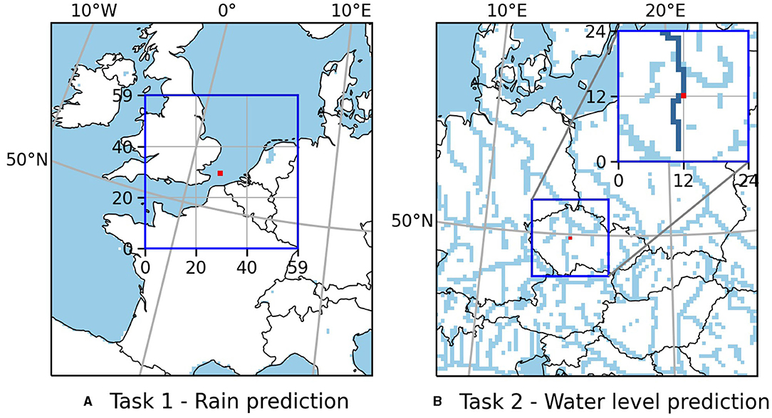
Figure 1. Set up of the two original prediction tasks. (A) Predict whether the precipitation averaged over the red 2 × 2 pixels target patch in the center of the 60 × 60 pixels input region exceeds 1 mm in the next 3 h. (B) Predict the water level at the red pixel given the water level 48 h earlier at the red pixel and the pixels upstream and downstream marked dark blue in the inset. Light blue indicates pixels with ponded water at the land surface during the entire simulation period (rivers, lakes, …).

A third example for the definition of a variant task is to consider a modification of the target variable. Later, for instance, we predict the water level at a location in a river given the water level in some specified segment of the river (see Figure 1B). As a variant task, we consider the same segment of the river but shift the target location by τ pixels along the river (see Figure 2B). As original and variant descriptions $\overrightarrow{d},\overrightarrow{d^v}\in {ℝ}^d$, we consider a measure of the average importance of each pixel in the specified river segment for the predictions of the original model and the variant model, respectively. In this case, we assume that causal relations are shifted along the river by the same distance as the target location is (i.e., by τ pixels). Hence, we choose to compute the dimensionwise distance between the original description $\overrightarrow{d}$ and the variant description $\overrightarrow{d^v}$ shifted by τ dimensions (i.e., we consider the distance $|{\overrightarrow{d}}_j-{\overrightarrow{d^v}}_{j+\tau }|$ for all j for that j+τ ∈ {1, …, d}). Using the above formalism, this corresponds to defining the boolean vectors ${(\overrightarrow{I_j})}_i={(\overrightarrow{I_j^v})}_{i+\tau }={\delta }_{ji}$ and the distance functions $dis{t}_j(\overrightarrow{d},\overrightarrow{d^v})=|{\overrightarrow{d}}_j-{\overrightarrow{d^v}}_{j+\tau }|$ for all j = 1, …, d for that j+τ ∈ {1, …, d}. Now, $dis{t}_j(\overrightarrow{d},\overrightarrow{d^v})\gg 0$ indicates that the part $\overrightarrow{d}(\overrightarrow{I_j})={\overrightarrow{d}}_j$ of the original description, or the part $\overrightarrow{d^v}(\overrightarrow{I_j^v})={\overrightarrow{d^v}}_{j+\tau }$ of the variant description, reflects spurious relations.

FIGURE 2

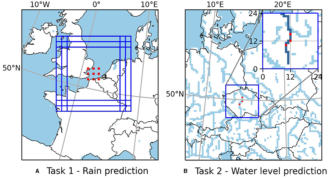
Figure 2. Location variant tasks. (A) Original target patch (center) with its input region and eight additional target patches and their (overlapping) input regions. (B) Original target location (center) and two additional target locations closely upstream and downstream.

In this example, it might be more realistic to assume that causal relations are not shifted along the river by exactly τ pixels, but that the shift distance depends on the flow velocity and potentially further influences. The proposed formalism allows to take this into account by varying the definition of $\overrightarrow{I_j}$, $\overrightarrow{I_j^v}$ and dist_j. Suppose, for instance, that the flow velocity around the original target location is twice as high as around the shifted target location. In this case, we might assume that the sum of importance of the two pixels upstream of the original target location should be identical to the importance of the single pixel upstream of the shifted target location. Hence, we might decide to consider ${(\overrightarrow{I_j})}_i={\delta }_{ji}+{\delta }_{j-1,i}$, ${(\overrightarrow{I_j^v})}_{i+\tau }={\delta }_{ji}$ (as above), and $dis{t}_j(\overrightarrow{d},\overrightarrow{d^v})=|({\overrightarrow{d}}_j+{\overrightarrow{d}}_{j-1})-{\overrightarrow{d^v}}_{j+\tau }|$, where the index j corresponds to the original target location. In this case, $dis{t}_j(\overrightarrow{d},\overrightarrow{d^v})\gg 0$ indicates that the part $\overrightarrow{d}(\overrightarrow{I_j})$ (corresponding to ${\overrightarrow{d}}_j$ and ${\overrightarrow{d}}_{j-1}$) of the original description, or the part $\overrightarrow{d^v}(\overrightarrow{I_j^v})={\overrightarrow{d^v}}_{j+\tau }$ of the variant description, reflects spurious relations.

In general, however, it is difficult to take variations of flow velocity and further influences into account when defining $\overrightarrow{I_j}$, $\overrightarrow{I_j^v}$ and dist_j. This is for example due to unavailable data on flow velocity and nonlinear behavior (e.g., that the sum of importance of the two pixels upstream of the original target location should be identical to the importance of the single pixel upstream of the shifted target location if the flow velocity in the respective river segment is twice as high, likely represents a too strong assumption on linearity). We will come back to this in the discussion of the results.

Let us return to the formal definition of the variant approach. The first step was to define a variant task. The second step consists of training a separate instance of the original model (a variant model) on this task and computing a variant description. The third step of the approach consists of comparing original and variant description and evaluating $dis{t}_j(\overrightarrow{d},\overrightarrow{d^v})\gg 0$ for all j = 1, …, m. If $dis{t}_j(\overrightarrow{d},\overrightarrow{d^v})\gg 0$ for some j ∈ {1, …, m}, the user infers that $\overrightarrow{d}(\overrightarrow{I_j})$ or $\overrightarrow{d^v}(\overrightarrow{I_j^v})$ reflects spurious relations. Note that the converse is not possible, i.e., if $dis{t}_j(\overrightarrow{d},\overrightarrow{d^v})\approx 0$, the user cannot infer that $\overrightarrow{d}(\overrightarrow{I_j})$ reflects causal relations (as it might be that both $\overrightarrow{d}(\overrightarrow{I_j})$ and $\overrightarrow{d^v}(\overrightarrow{I_j^v})$ reflect spurious relations). Note further that the specification of the condition $dis{t}_j(\overrightarrow{d},\overrightarrow{d^v})\gg 0$ should in general take into account the specific original and variant task, the choice of the distance function dist_j, and the certainty of the assumed stability or systematic variation, respectively, of causal relations. Moreover, in case the user does not need a binary identification of parts of $\overrightarrow{d}$ that reflect spurious relations, it might be better not to consider the binary condition $dis{t}_j(\overrightarrow{d},\overrightarrow{d^v})\gg 0$, but to consider raw values $dis{t}_j(\overrightarrow{d},\overrightarrow{d^v})$, where higher distances indicate a higher probability that $\overrightarrow{d}(\overrightarrow{I_j})$ or $\overrightarrow{d^v}(\overrightarrow{I_j^v})$ reflects spurious relations.

For all variant tasks defined in this work, the expression $dis{t}_j(\overrightarrow{d},\overrightarrow{d^v})$ corresponds to the relative distance between a single component ${\overrightarrow{d}}_{j_1}$ of an original description and a single component ${\overrightarrow{d^v}}_{j_2}$ of a corresponding variant description, i.e., it takes the form

$\begin{array}{ll}dis{t}_j(\overrightarrow{d},\overrightarrow{d^v})=\frac{|{\overrightarrow{d}}_{j_1}-{\overrightarrow{d^v}}_{j_2}|}{|{\overrightarrow{d}}_{j_1}|+|{\overrightarrow{d^v}}_{j_2}|+\epsilon },& (1)\end{array}$

with some regularization parameter ε≥0. By considering relative distances rather than absolute distances, we define, for instance, that ${\overrightarrow{d}}_{j_1}=100$, ${\overrightarrow{d^v}}_{j_2}=101$ agree better than ${\overrightarrow{d}}_{j_1}=1$, ${\overrightarrow{d^v}}_{j_2}=2$, or, in other words, in the latter case it is more likely that the value ${\overrightarrow{d}}_{j_1}$ or the value ${\overrightarrow{d^v}}_{j_2}$ reflects spurious relations. Further, an advantage of considering relative distances is that all distances lie between zero and one (when neglecting ε) which allows to apply a threshold t ∈ (0, 1) to specify the condition $dis{t}_j(\overrightarrow{d},\overrightarrow{d^v})\gg 0$ and to mark all parts $\overrightarrow{d}(I_j)$ of the original description as spurious for which $dis{t}_j(\overrightarrow{d},\overrightarrow{d^v})>t$. In this study, we use t = 0.5 as threshold and ε = 1e−3 as regularization parameter. Choosing a smaller threshold, more values are marked as spurious (with all values marked as spurious for t = 0), and choosing a larger threshold, fewer values are marked as spurious (with no values marked as spurious for t = 1) by definition. For the examples considered below, t = 0.5 seems to be a good choice.

2.2. Illustrative Tasks

In this section, we define two prediction tasks and corresponding variant tasks that illustrate the proposed variant approach. We chose simplified tasks and global descriptions of the learned functions to be able to decide whether parts of the descriptions that the variant approach marks as spurious do indeed reflect spurious relations. The data underlying both tasks is 3-hourly data at 412 × 424 pixels over Europe. The data was obtained from a long-term (January 1996–August 2018), high-resolution (≈12.5 km) simulation (Furusho-Percot et al., 2019) performed with the Terrestrial Systems Modeling Platform (TSMP), a fully integrated groundwater-soil-vegetation-atmosphere modeling system (Gasper et al., 2014; Shrestha et al., 2014). Note that the statistical models and interpretation methods applied in this work are described in section 2.3.

2.2.1. Task 1 – Rain prediction

In the first example, we predict the occurrence of rain at a 2 × 2 pixels target patch, given the geopotential fields at 500, 850, and 1,000 hPa in the 60 × 60 pixels neighborhood (see Figure 1A). We model this as a classification task and define that rain occurred, if the precipitation averaged over the target patch exceeds 1 mm in the following 3 h. Previous works (Larraondo et al., 2019; Pan et al., 2019) have used CNNs to predict precipitation given geopotential fields to improve the parameterization of precipitation in numerical weather prediction models. Thus, apart from the simplifications of only one target location and a binary target, this is a realistic prediction task.

As statistical models, we consider a logistic regression model and two convolutional neural networks (CNNs) of different depth and complexity. As description of the function that the logistic regression model learns, we consider the absolute values of the model weights averaged over the pressure level axis. As descriptions of the functions that the CNNs learn, we consider saliency maps averaged over the pressure level axis and over all training samples. These descriptions can be seen as measures of the average importance of each pixel in the 60 × 60 pixels input region for the predictions of the models (for details see the respective sections below).

To identify whether parts of the descriptions reflect spurious relations that the models learned, we compute descriptions for variant models trained on three types of variant tasks. The first type (later referred to as sampling type) considers the same task, but a modified training set obtained by randomly sampling 70 % of the original training set without replacement. In this case, we assume that all causal relations remain stable. Hence, we compute the pixelwise distance between original and variant descriptions. We repeat the sampling procedure 10 times obtaining 10 variant tasks of this type. The second type of variant tasks (later referred to as size type) considers the same task but the input variables in the 80 × 80 pixels neighborhood of the target patch. In this case, we assume that causal relations between pixels in the 60 × 60 pixels neighborhood and rain events at the target patch remain stable when enlarging the considered neighborhood by 10 pixels on each side. Hence, we compute the pixelwise distance between the original descriptions and the central 60 × 60 pixels of the variant descriptions. The third type of variant task (later referred to as location type) considers the same task but for eight different target patches obtained by moving the original target patch by five pixels to the left or right, and up or down. The input regions are shifted accordingly (see Figure 2A). In this case, we assume again that all causal relations remain stable. Hence, we again compute the pixelwise distance between original and variant descriptions.

Note that to compute the variant descriptions for the functions that separate instances of the CNNs learn when trained for different target locations, we average the saliency maps over all training samples from the original task. This is because the distribution $p(\overrightarrow{x})$ of geopotential fields differs at different locations. Thus, if we averaged the saliency maps for a variant CNN over all training samples from a variant task, the obtained variant description would differ from the original description even if original and variant models learned the exact same function relating geopotential fields and rain events.

We obtained the geopotential fields and precipitation data from the aforementioned simulation. We selected the geopotential fields in the considered input regions and created the binary rain event time series for the corresponding target patches. Next, we split the time series using the first 56,000 time steps as training candidates and the last 10,183 time steps as validation candidates. Finally, training and validation sets were obtained by selecting all time steps followed by a rain event at the considered target patch and an equal amount of randomly chosen additional time steps for non-rain events from the training and validation candidates, respectively. This resulted in balanced training and validation sets of a total of approximately 10,000 time steps for each target patch. Handling strongly unbalanced data sets as it would be necessary without such a selection of time steps is out of scope for this work.

2.2.2. Task 2 – Water Level Prediction

As a second example, we predict the water level at a location in a river, given the water level in a specific segment of the river 48 h earlier (see Figure 1B).

As statistical models, we consider a linear regression model and a multilayer perceptron (MLP). As description of the function that the linear regression model learns, we consider as in Task 1 the absolute values of the model weights. For the MLP, we consider again the saliency maps averaged over all training samples. Analogously to Task 1, these descriptions can be seen as measures of the average importance of each pixel in the considered river segment for the predictions of the models (for details see the respective sections below).

To identify whether parts of the descriptions reflect spurious relations that the models learned, we compute descriptions for variant models trained on two types of variant tasks. The first type (later referred to as sampling type) considers the same task, but a modified training set obtained by randomly sampling 70 % of the original training set without replacement. In this case, we assume that all causal relations remain stable. Hence, we compute the pixelwise distance between original and variant descriptions. We repeat the sampling procedure 10 times obtaining 10 variant tasks of this type. The second type of variant tasks (later referred to as location type) considers the same river segment as input, but target locations closely upstream and downstream of the original target location (see Figure 2B). In this case, we assume that causal relations are shifted along the river by the same distance as the target location is. Hence, we compute the pixelwise distance between the original description $\overrightarrow{d}$ and the variant description $\overrightarrow{d^v}$ shifted by τ pixels, where τ is the number of pixels that the target location was shifted (i.e., we consider the distance $|{\overrightarrow{d}}_j-{\overrightarrow{d^v}}_{j+\tau }|$ for all j for that j+τ ∈ {1, …, d}).

We obtained the water level data from the aforementioned simulation. In contrast to Task 1, this task is not a classification but a regression task; discarding time steps to obtain a balanced data set is not necessary. Hence, we use water level data for all 64,240 3-hourly time steps between January 1996 and December 2017. We randomly selected the years 1997, 2004, 2008, and 2015 as test data, covering the whole period of time, and use the remaining years to train the models.

2.3. Statistical Models and Descriptions

In this section, we present the statistical models used in this study. Further, we describe saliency maps, the interpretation method applied to obtain descriptions of the functions that the neural networks (MLP and CNNs) learn. Note that for the considered examples, layerwise relevance propagation (LRP) and Grad-CAM give very similar results to saliency maps. The section is ordered with respect to the complexity of the described methods from simple to complex.

2.3.1. Linear Regression

Given training samples ${({\overrightarrow{x}}_i,y_i)}_{i=1}^n$ with ${\overrightarrow{x}}_i\in {ℝ}^N$, y_i ∈ ℝ, a linear regression model learns a function f:ℝ^N → ℝ of the form

$\begin{array}{ll}f(\overrightarrow{x})={\beta }_0+{\overrightarrow{x}}^T·\overrightarrow{\bar{\beta }},& (2)\end{array}$

where $\overrightarrow{\beta }=({\beta }_0,\overrightarrow{\bar{\beta }})=({\beta }_0,{\beta }_1,\dots ,{\beta }_N)\in {ℝ}^{N+1}$ are the weights of the model. Those weights are obtained by minimizing the squared error on the training set

$\begin{array}{ll}{\displaystyle \sum _{i=1}^n}{(f({\overrightarrow{x}}_i)-y_i)}^2.& (3)\end{array}$

Optionally, a regularization term can be added to the objective. We calculate the minimizing weights $\overrightarrow{\beta }$ using the implementation of scikit-learn (Pedregosa et al., 2011). In our case, the inputs ${\overrightarrow{x}}_i$ are elements of ℝ³⁰ representing the water level at the 30 pixels in the considered river segment (see Figure 1B) and the targets y_i ∈ ℝ represent the water level at the target pixel 48 h later.

As description of the function that a linear regression model learned, we consider the absolute values of the weights $\overrightarrow{\bar{\beta }}$. This can be seen as a measure of the average importance of each pixel in the river segment for the predictions of the model (Molnar, 2019).

2.3.2. Logistic Regression

Given the task to predict a binary target y ∈ {0, 1} from an input $\overrightarrow{x}\in {ℝ}^N$, a logistic regression model yields

$\begin{array}{ll}P(y=1|\overrightarrow{x},\overrightarrow{\beta })=\frac{1}{1+exp(-({\beta }_0+{\overrightarrow{x}}^T·\overrightarrow{\bar{\beta }}))},& (4)\end{array}$

where $\overrightarrow{\beta }=({\beta }_0,\overrightarrow{\bar{\beta }})=({\beta }_0,{\beta }_1,\dots ,{\beta }_N)\in {ℝ}^{N+1}$ are the weights of the model. These weights are obtained by minimizing the function

$\begin{array}{ll}-{\displaystyle \prod _{i=1}^n}P{(y_i=1|{\overrightarrow{x}}_i,\overrightarrow{\beta })}^{y_i}·{(1-P(y_i=1|{\overrightarrow{x}}_i,\overrightarrow{\beta }))}^{1-y_i}+\lambda R(\overrightarrow{\beta })& (5)\end{array}$

with respect to $\overrightarrow{\beta }$. Here, ${({\overrightarrow{x}}_i,y_i)}_{i=1}^n$ are training samples with ${\overrightarrow{x}}_i\in {ℝ}^N,y_i\in \left\{0,1\right\}$, and $\lambda R(\overrightarrow{\beta })$ is a regularization term. The product represents the probability with that – according to the logistic regression model with weights $\overrightarrow{\beta }$ – the targets y_i are observed given the input samples ${\overrightarrow{x}}_i$. Thus, minimizing the negative product with respect to $\overrightarrow{\beta }$ corresponds to finding the $\overrightarrow{\beta }$ for that the highest probability is assigned to observing the targets y_i given the inputs ${\overrightarrow{x}}_i$ from the training set. We use scikit-learn (Pedregosa et al., 2011) (solver “liblinear”) to approximate the minimizing weights $\overrightarrow{\beta }$. In our case, the inputs ${\overrightarrow{x}}_i$ are the geopotential fields at 500, 850 and 1000 hPa flattened to vectors in ℝ^3·60·60 and the targets y_i ∈ {0, 1} represent whether a rain event took place or not.

As description of the function that a logistic regression model learned, we consider the weights $\overrightarrow{\bar{\beta }}$. We reshape the vector $\overrightarrow{\bar{\beta }}$ to the shape of the original input, 3 × 60 × 60, take the absolute value and build an average over the first (pressure level) axis. This can be seen as a measure of the average importance of each pixel in the 60 × 60 pixels input region for the predictions of the model (Molnar, 2019).

2.3.3. Multilayer Perceptron

Multilayer Perceptrons (MLPs), also referred to as fully-connected neural networks, are feedforward artificial neural networks. They are composed of one or more hidden layers and an output layer. Each layer comprises several neurons. Each neuron in the first hidden layer builds a weighted sum of all input variables, while each neuron in the subsequent layers builds a weighted sum of the outputs of the neurons in the respective previous layer. In case of a neuron in a hidden layer, the sum is passed through a nonlinear activation function and forms the input to the next layer. In case of a neuron in the output layer, the sum is optionally passed through a nonlinear activation function and forms the output of the neural network. The weights of the MLP are learned by minimizing a loss function on training samples ${({\overrightarrow{x}}_i,{\overrightarrow{y}}_i)}_{i=1}^n$, ${\overrightarrow{x}}_i\in {ℝ}^N,{\overrightarrow{y}}_i\in {ℝ}^K$, using backpropagation (LeCun et al., 2012).

In our case, the inputs to the MLP are elements $\overrightarrow{x}$ of ℝ³⁰ representing the water level at the 30 pixels in the considered river segment (see Figure 1B). The targets y_i ∈ ℝ represent the water level at the target pixel 48 h later. Section 2.3.5 describes how we obtained a description of the function that the MLP learned. The network and training of the MLP were implemented using the deep learning library Pytorch (Paszke et al., 2019). A detailed description of the used architecture and training procedure can be found in the Supplementary Material.

2.3.4. Convolutional Neural Networks

Convolutional Neural Networks (CNNs) are frequently employed DL models designed to process stacks of multiple arrays containing spatially structured data. This can, for example, be a stack of 2-dimensional arrays for an RGB image (${\overrightarrow{x}}_i\in {ℝ}^{3\times \mathrm{\text{height}}\times \mathrm{\text{width}}}$) or, as in our case, a stack of 2-dimensional geopotential fields at different pressure levels in the atmosphere (${\overrightarrow{x}}_i\in {ℝ}^{3\times 60\times 60}$). Typically, a CNN consists of three types of layers: convolutional layers, pooling layers and fully-connected layers. In the following short review of the typical CNN layers, we consider the case of one or multiple 2-dimensional input arrays. A generalization of the concepts to N-dimensional input arrays is straightforward.

The input to a convolutional layer is a stack of c_in 2-dimensional arrays and its output is a stack of c_out 2-dimensional arrays. The convolutional layer is characterized by c_out kernels, which are 3-dimensional tensors of shape c_in×k×k, where the kernel size k is usually between 1 and 7. The output of the layer are the c_out 2-dimensional arrays obtained by convolving the input with each kernel along the last two dimensions. Usually, a convolutional layer is directly followed by a nonlinear activation function which is applied elementwise to the layer's output. In contrast to a fully-connected layer, a convolutional layer preserves the spatial structure of the input: only neurons in a neighborhood defined by the kernel size influence the output of a specific neuron.

As for convolutional layers, the input to a pooling layer is a stack of c_in 2-dimensional arrays of shape n×m. Pooling layers reduce the dimensionality of the 2-dimensional arrays creating invariances to small shifts and distortions. A typical form of pooling is max-pooling with a kernel size of two. This reduces the resolution along both axes of each of the c_in 2-dimensional arrays by a factor of two, picking always the maximum value of a 2 × 2 patch of the original array. Thus, the output of this pooling layer is a stack of c_out = c_in 2-dimensional arrays of shape $\frac{n}{2}\times \frac{m}{2}$.

After several alternating convolutional and pooling layers which extract features of increasing complexity, the resulting c 2-dimensional arrays are flattened into a single vector and one or more fully-connected layers, as described for the MLP, follow. The weights for the kernels in the convolutional layers and the fully-connected layers are learned by minimizing a loss function on training samples ${({\overrightarrow{x}}_i,{\overrightarrow{y}}_i)}_{i=1}^n$, ${\overrightarrow{x}}_i\in {ℝ}^N,{\overrightarrow{y}}_i\in {ℝ}^K$, using backpropagation (LeCun et al., 2012). To prevent CNNs from overfitting, dropout regularization (Srivastava et al., 2014) and batch normalization (Ioffe and Szegedy, 2015) are commonly employed techniques.

In our case, the inputs ${\overrightarrow{x}}_i$ are the geopotential fields at 500, 850 and 1000 hPa, ${\overrightarrow{x}}_i\in {ℝ}^{3\times 60\times 60}$. The targets y_i ∈ {0, 1} represent whether a rain event took place or not. We consider two convolutional neural networks of different depth and complexity. CNN1 is a shallow CNN with only two convolutional layers followed by a single fully-connected layer. CNN2 is a commonly employed, much deeper CNN architecture called resnet18 (He et al., 2016) for which the last fully-connected layer was adapted to have only two output neurons to fit our binary prediction task. Section 2.3.5 describes how we obtained descriptions of the functions that the CNNs learned. The networks and training were implemented using the deep learning library Pytorch (Paszke et al., 2019). A detailed description of the used CNN architectures and training procedure can be found in the Supplementary Material.

2.3.5. Saliency Maps

A common subgroup of interpretation methods providing descriptions of the functions that neural networks (NNs) learn, are methods that assign an importance to each dimension of individual input samples $\overrightarrow{x}\in {ℝ}^N$ (local feature importance scores), see e.g., Samek et al., 2021. Among the most employed and well-known methods for that purpose are saliency maps (Simonyan et al., 2014), layerwise relevance propagation (LRP) (Bach et al., 2015) and Grad-CAM (Selvaraju et al., 2017). In the examples presented in this work, all three methods yield similar results. Therefore and for the sake of brevity, we focus on saliency maps (although e.g., Montavon et al., 2018 argue that saliency maps provide a bad measure of feature importance because they indicate how the prediction of a model changes when the value of a feature is changed, rather than indicating what makes the model make a prediction).

Note that in contrast to the weights of linear and logistic regression models, saliency maps are local descriptions of the learned functions, i.e., the importance assigned to an input dimension (in our case an input pixel) depends on the input sample $\overrightarrow{x}$. To get a global description of the learned function and a measure of the average importance of each input pixel, we average the saliency maps over all training samples.

In the rain prediction task, the NN defines an (almost everywhere) differentiable function f that maps geopotential fields $\overrightarrow{x}\in {ℝ}^{3\times 60\times 60}$ to probabilities $f(\overrightarrow{x})=y\in (0,1)$ that a rain event occurs. The partial derivative

$\begin{array}{ll}{w}_{cij}(\overrightarrow{x})=\frac{\partial f}{\partial x_{cij}}(\overrightarrow{x}),c=1,2,3,i,j=1,\dots ,60& (6)\end{array}$

indicates how a small perturbation of the c-th geopotential field at pixel (i, j) affects the prediction of the NN. The saliency map

$\begin{array}{ll}{M}_{ij}(\overrightarrow{x})=\frac{1}{3}{\displaystyle \sum _{c=1}^3}|w_{cij}(\overrightarrow{x})|,i,j=1,\dots ,60& (7)\end{array}$

considers the absolute value of the partial derivatives averaged over the pressure level axis to obtain for each pixel in the 60 × 60 pixels input region a measure of its importance for the model's prediction for sample $\overrightarrow{x}$.

In the water level prediction task, the neural network maps water levels $\overrightarrow{x}\in {ℝ}^{30}$ to a water level prediction $f(\overrightarrow{x})=y\in ℝ$. The saliency map

$\begin{array}{ll}{M}_i(\overrightarrow{x})=\left|w_i(\overrightarrow{x})\right|=\left|\frac{\partial f}{\partial x_i}(\overrightarrow{x})\right|,i=1,\dots ,30& (8)\end{array}$

provides for each pixel in the considered river segment a measure of its importance for the model's prediction for sample $\overrightarrow{x}$.

3. Results and Discussion

3.1. Task 1 – Rain Prediction

Figure 3A shows the description $\overrightarrow{d}$ of the function that CNN1 learned when it was trained on the original rain prediction task. Remember that the considered description is a measure of the average importance of each pixel in the 60 × 60 pixels input region for the predictions of the model. Our objective is to apply the variant approach to identify parts of the description that reflect spurious relations. To that purpose, we defined several variant tasks above. As a next step, we computed the corresponding variant descriptions, i.e., the descriptions of the functions that separate instances of CNN1 learned when trained on these variant tasks. For illustration, Figure 4 shows the original description (center, same as Figure 3A) and the variant descriptions $\overrightarrow{d^{v_i}},i=1,\dots ,8$, obtained for the eight location variant tasks (see Figure 2A).

FIGURE 3

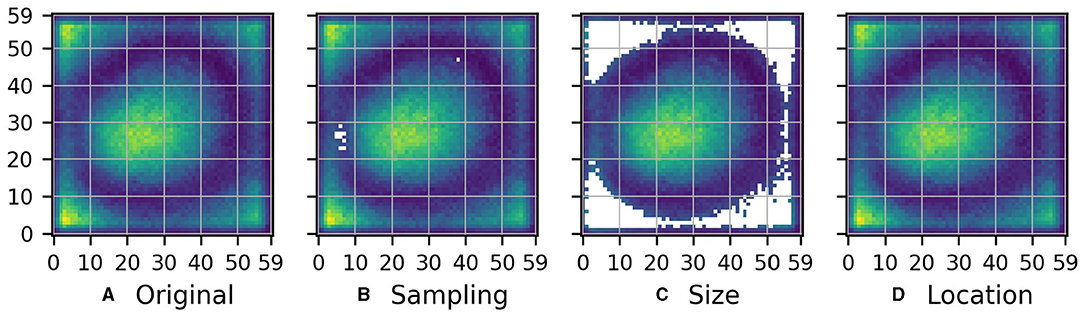
Figure 3. (A) Description $\overrightarrow{d}$ of the function that CNN1 learned when it was trained on the original rain prediction task (see Figure 1A). The description is a measure of the average importance of each pixel in the 60 × 60 pixels input region for the predictions of the model. Yellow color indicates high and blue color low importance. (B–D) As (A), but pixels for which the relative distance between the original description $\overrightarrow{d}$ and one of the variant descriptions $\overrightarrow{d^{v_i}}$ obtained for the sampling, size, and location variant tasks, respectively, exceeds the threshold of t = 0.5, are masked.

FIGURE 4

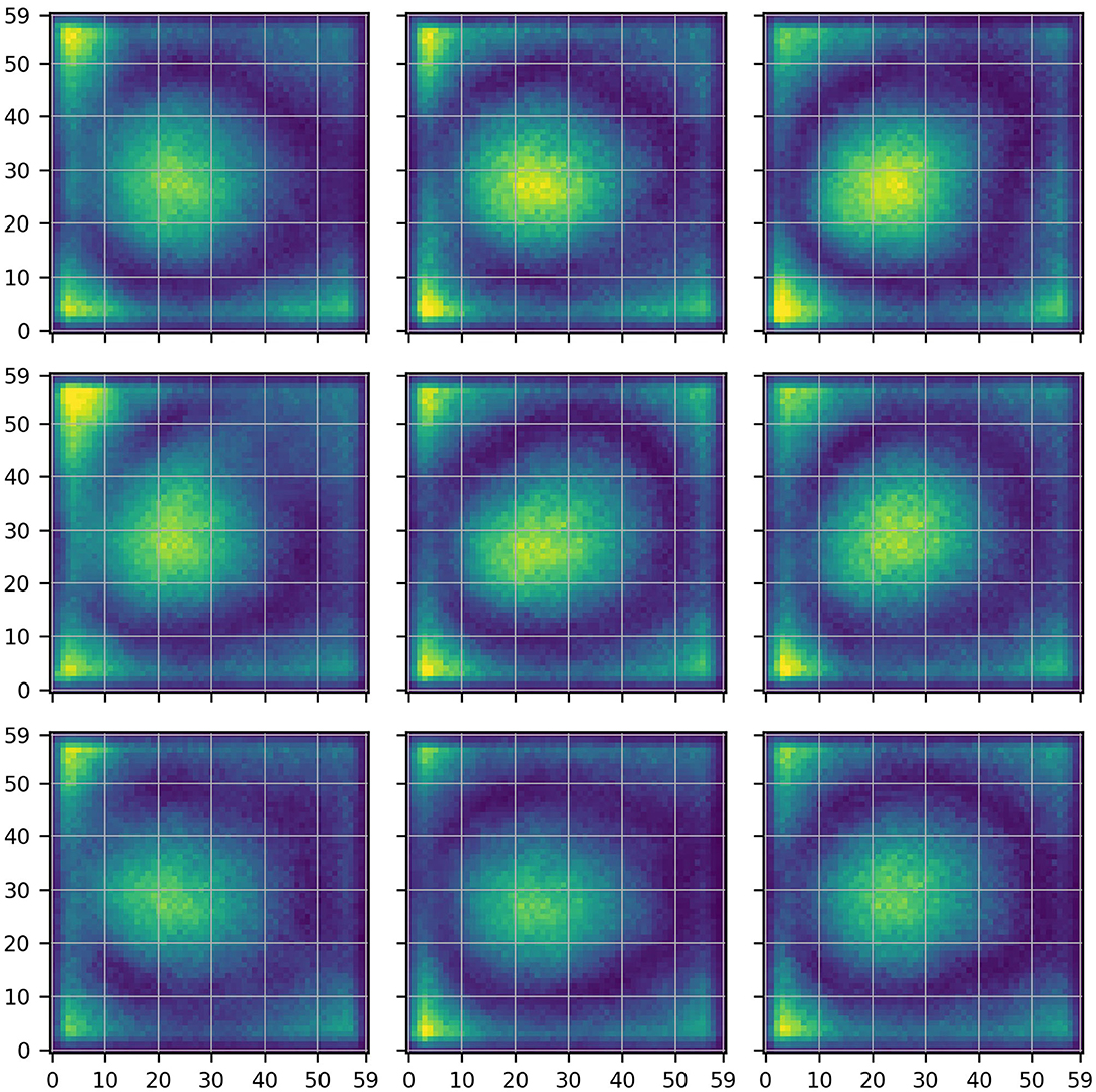
Figure 4. Descriptions obtained when training separate instances of CNN1 for the nine different locations depicted in Figure 2A. Each description is a measure of the average importance of each pixel in the 60 × 60 pixels input region for the predictions of the respective instance of CNN1. Yellow color indicates high and blue color low importance. The central location is the original target location, hence the central description identical to Figure 3A.

For each of these variant descriptions $\overrightarrow{d^{v_i}}\in {ℝ}^{60\times 60},i=1,\dots ,8$, we evaluated the pixelwise relative distance to the original description $\overrightarrow{d}\in {ℝ}^{60\times 60}$ (see Equation 1), and masked all pixels of the original description $\overrightarrow{d}$ for which this distance exceeds the threshold of t = 0.5 for any $\overrightarrow{d^{v_i}}$. The resulting masked version of $\overrightarrow{d}$ is shown in Figure 3D. Note that in this case, there is no pixel for which the relative distance between original description and any of the variant descriptions exceeds 0.5, hence Figure 3D is identical to Figure 3A. Analogously to Figures 3B,D shows the masked version of $\overrightarrow{d}$ obtained when masking all pixels for which the pixelwise relative distance between $\overrightarrow{d}$ and one of the variant descriptions $\overrightarrow{d^{v_i}}$ obtained for the sampling variant tasks exceeds 0.5. We observe that some pixels in the west of the inner area of importance are masked, indicating that the inner area of importance might actually extend further to the west. Figure 3C shows the masked version of $\overrightarrow{d}$ obtained when masking all pixels for which the pixelwise relative distance between $\overrightarrow{d}$ and the central 60 × 60 pixels of the variant description $\overrightarrow{d^{v_i}}$ obtained for the size variant task exceeds 0.5. Notably, all the boundary pixels with high values in Figure 3A are masked, indicating that these values likely reflect spurious relations.

Figure 5 shows the same as Figure 3 but for CNN2. Only few pixels are masked for the sampling and location variant tasks. However, the mask obtained for the size variant task indicates that the checkerboard pattern in the original description $\overrightarrow{d}$, which is shown in Figure 5A, likely reflects spurious relations. Note that this checkerboard pattern is indeed a known artifact of strided convolutions and max-pooling layers used in CNN2 (Odena et al., 2016).

FIGURE 5

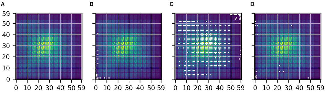
Figure 5. Same as Figure 3 but for CNN2. (A) Original. (B) Sampling. (C) Size. (D) Location.

Figure 6 shows the same as Figures 3 and 5 but for the logistic regression model. For the sampling variant tasks, large parts of the original description $\overrightarrow{d}$ are masked. This indicates that these parts likely reflect spurious relations. For the size variant task, on the other side, only few pixels are masked. Lastly, for the location variant tasks, nearly all pixels are masked. This indicates that the original description $\overrightarrow{d}$ shown in Figure 6A likely reflects spurious relations only.

FIGURE 6

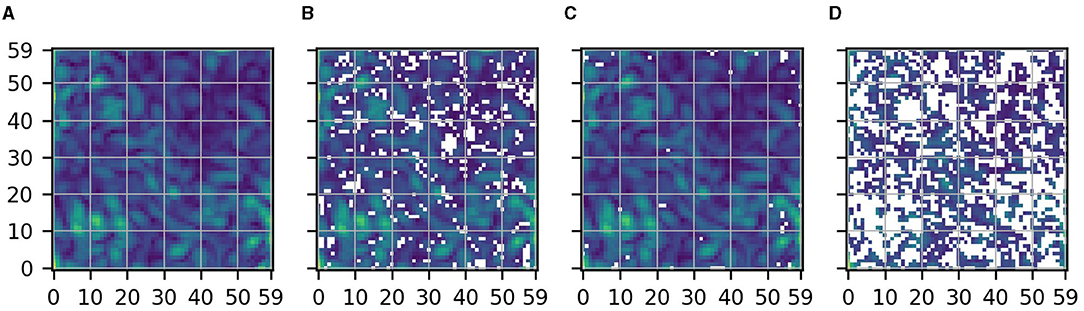
Figure 6. Same as Figure 3 but for the logistic regression model. (A) Original. (B) Sampling. (C) Size. (D) Location.

For this task, we know that the physical importance of a pixel averaged over a long time period decreases with the pixel's distance to the central target patch. Further, due to the predominantly westerly winds, the average physical importance of pixels is slightly shifted to the west. Given this knowledge, we can confirm that the variant approach successfully identified all pixels in Figures 3A, 5A, 6A which reflect spurious relations. Note that the sampling approach alone (see Figures 3B, 5B, 6B), which is the commonly applied method, is not sufficient to identify all pixels reflecting spurious relations.

Note further that the examples emphasize once again the following: even if parts of a description are not indicated as spurious by any considered variant task, we cannot conclude that they reflect causal relations. Imagine, for instance, that we had only considered the size variant task. For this variant task and the logistic regression model, only a small number of pixels is masked although Figure 6A seems to exclusively reflect spurious relations. Hence, variant tasks can only indicate parts of an original description as likely reflecting spurious relations and do not allow for any direct inference about other parts of the description. Nevertheless, this can be useful already.

3.2. Task 2 – Water Level Prediction

Figure 7A shows the description $\overrightarrow{d}$ of the function that the MLP learned when it was trained on the original water level prediction task. Remember that the considered description is a measure of the average importance of each pixel in the considered river segment for the predictions of the model. Our objective is to apply the variant approach to identify parts of the description that reflect spurious relations. To that purpose we computed the variant descriptions $\overrightarrow{d^{v_i}}$ for all sampling and location variant tasks, and masked all pixels of $\overrightarrow{d}$ for which the relative distance between the original description $\overrightarrow{d}$ and one of the (shifted) variant descriptions exceeds the threshold of t = 0.5. The resulting masked versions of Figure 7A are shown in Figures 7B, C.

FIGURE 7

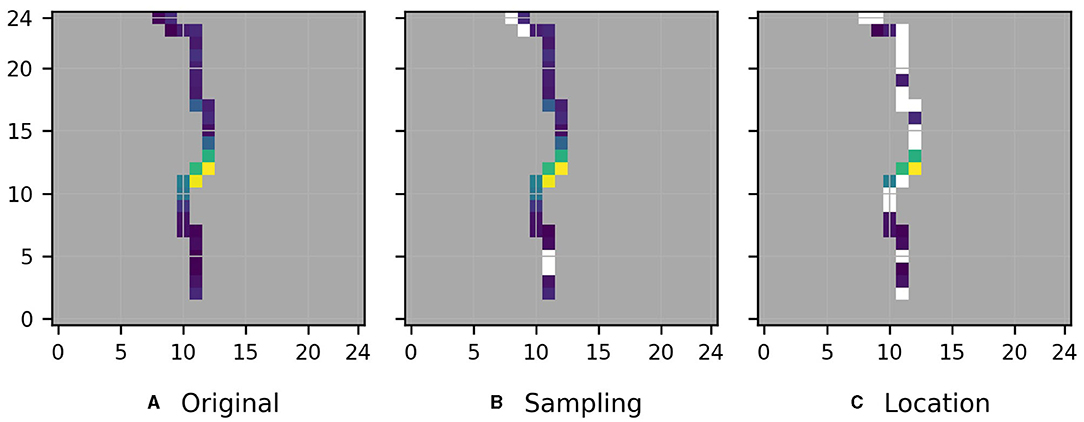
Figure 7. (A) Description $\overrightarrow{d}$ of the function that the MLP learned when it was trained on the original water level prediction task (see Figure 1B). The description is a measure of the average importance of each pixel in the considered river segment for the predictions of the model. Yellow color indicates high and blue color low importance. (B,C) As (A), but pixels for which the relative distance between the original description $\overrightarrow{d}$ and one of the sampling and (shifted) location variant descriptions $\overrightarrow{d^{v_i}}$, respectively, exceeds the threshold of t = 0.5, are masked. Gray marks pixels outside the considered river segment.

For this task, we know that the development of the water level at the target location depends only on the water level closely upstream and downstream. Hence, Figure 7A is [apart from the moderately high importance of pixel (11,17)] close to our understanding of the physical importance of the considered pixels. Nevertheless, especially in Figure 7C, many of the pixels further upstream and downstream of the target location are masked, i.e., the variant approach indicates (mistakenly) that the low feature importance of these pixels likely reflects spurious relations. We suspect that this happened because we considered relative rather than absolute distances between original and variant descriptions (see Equation 1), which can cause two small values to have a large distance which in turn causes the corresponding pixel to be mistakenly masked as spurious. Apart from pixels with low feature importance, also pixel (11,11) closely upstream of the original target location seems to be mistakenly masked as spurious in Figure 7C. We suspect that this is due to our assumption that causal relations are shifted along the river by the exact same number of pixels as the target location is. While this assumption enables us to simply consider pixelwise relative distances between original description $\overrightarrow{d}$ and shifted variant descriptions $\overrightarrow{d^{v_i}}$ (see section 2), it might be overly simplified as for example the flow velocity at different locations in the river might differ, and the river might cross some pixels diagonally and others straight.

Here, a visual assessment of the individual variant descriptions seems to be superior to the formal evaluation of distances performed for Figure 7C because it allows a softer comparison between original and variant descriptions $\overrightarrow{d}$ and $\overrightarrow{d^{v_i}}$. Indeed, upon visual assessment of the location variant descriptions depicted in Figure 8, and with the assumption in mind that causal relations approximately reflect the shift of the target location, the only pixel in Figure 7A that we would mark as potentially reflecting spurious relations, is pixel (11,17).

FIGURE 8

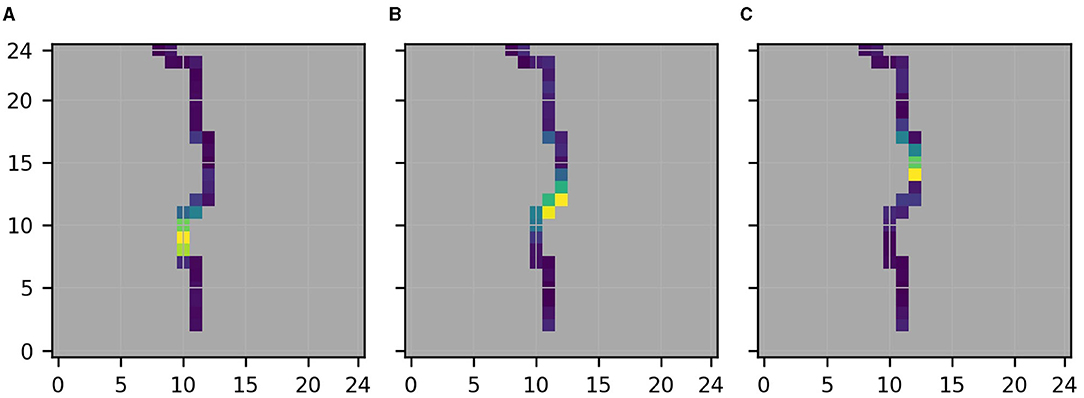
Figure 8. Descriptions of the functions that separate instances of the MLP learned when trained for the different target locations [From left to right the target location is at (10,10), (12,12), (12,15), see Figure 2B]. Note that (B) shows the same as Figure 7A. Gray marks pixels outside the considered river segment. (A) Lower target location. (B) Central target location. (C) Upper target location.

Figures 9, 10 show the same as Figures 7, 8 but for the linear regression model. In this case, the formal evaluation of distances between original and location variant descriptions performed for Figure 9C indicates that Figure 9A reflects spurious relations at nearly all pixels except from the target location and the neighboring pixel upstream. In this case, the formal evaluation agrees well with the visual assessment of the location variant descriptions depicted in Figure 10. Indeed, visual assessment of Figure 10 also indicates that the neighboring pixel upstream of the target location and maybe the target location itself are the only two pixels for which the assigned importance approximately reflects the shift of the target location between Figures 10A–C.

FIGURE 9

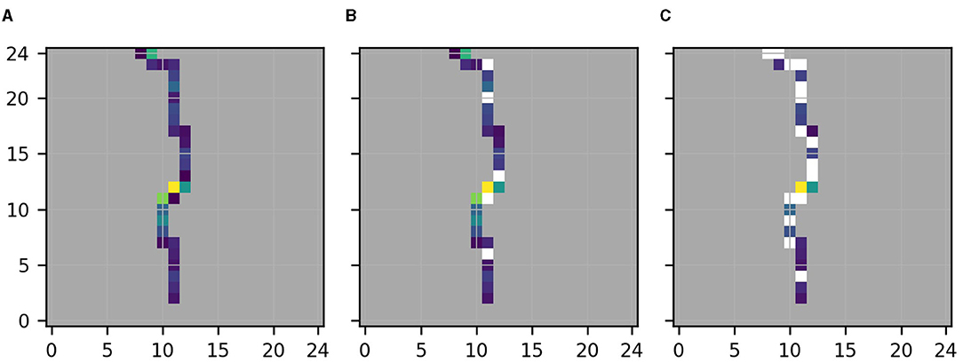
Figure 9. Same as Figure 7 but for the linear regression model. (A) Original. (B) Sampling. (C) Location.

FIGURE 10

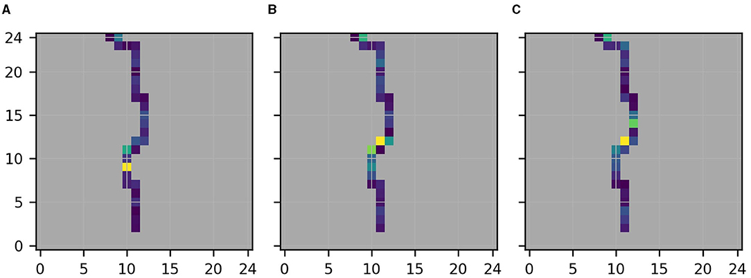
Figure 10. Same as Figure 8 but for the linear regression model. (A) Lower target location. (B) Central target location. (C) Upper target location.

4. Conclusions

Given a description $\overrightarrow{d}\in {ℝ}^d$ of the function that a statistical model learned during a training phase, we proposed a variant approach for the identification of parts of $\overrightarrow{d}$ that reflect spurious relations. We successfully demonstrated the approach and its superiority over pure sampling approaches with two illustrative hydrometeorological predictions tasks, various statistical models and illustrative descriptions. For the rain prediction task, where we assumed causal relations to remain stable between original and variant tasks, the formal evaluation of distances between original and variant descriptions enabled us to correctly identify all spurious relations that the statistical models learned. For the water level prediction task, where formally specifying the assumed variation of causal relations was more involved, we found the formal evaluation of distances to be of limited use. However, visual assessment enabled us again to correctly identify all spurious relations that the statistical models learned.

In this work, we considered simplified tasks and global descriptions of the learned functions to be able to decide whether parts of the descriptions that the variant approach identifies as spurious do indeed reflect spurious relations. This was necessary to evaluate the variant approach. However, we expect the approach to be beneficial for a wide range of more complex prediction tasks. Naming two possible applications outside the geosciences, it might be used to identify spurious relations reflected in (local) descriptions of functions that DL models trained on electroencephalography (EEG) data (Sturm et al., 2016) learned by comparing them to variant descriptions obtained for variant models trained for different (groups of) patients; or to automatically detect spurious relations reflected in (local) descriptions of functions that a DL model trained on a common image data set learned (Lapuschkin et al., 2019) by automatically comparing them to variant descriptions for variant models trained on different image data sets. Applications of the variant approach to more complex prediction tasks in the geosciences and beyond, and to local descriptions of the learned functions, are planned in future.

A challenge when applying the proposed variant approach may be to define variant tasks beyond random sampling of the training data. However, a data set is often composed of different sources constituting in themselves variants. Further, the modification of the rain prediction task, where we were able to identify parts of the original description as spurious by merely changing the size of the input region, indicates that even small modifications of the original prediction task can be useful.

Apart from the variant approach, which considers a fixed statistical model and modifications of an original prediction task, another approach for identifying spurious relations that a considered statistical model learned might be to compare the relations between input and target variables that different models learn when trained on the (fixed) prediction task. In such an approach, the degree of variation between models may differ from varying configurations in Monte-Carlo dropout, over random seeds for the weight initialization of otherwise identical models to completely different statistical models. Formalization and evaluation of this approach is out of scope of this work.

Data Availability Statement

The datasets presented in this study can be found in online repositories. Code for replication of the study is available at: https://datapub.fz-juelich.de/slts/t_tesch/.

Author Contributions

TT and SK designed the experiments. TT conducted the experiments, analyzed the results and prepared the manuscript with contributions from SK and JG. All authors contributed to the article and approved the submitted version.

Author Disclaimer

The content of the paper is the sole responsibility of the author(s) and it does not represent the opinion of the Helmholtz Association, and the Helmholtz Association is not responsible for any use that might be made of the information contained.

Conflict of Interest

The authors declare that the research was conducted in the absence of any commercial or financial relationships that could be construed as a potential conflict of interest.

Publisher's Note

All claims expressed in this article are solely those of the authors and do not necessarily represent those of their affiliated organizations, or those of the publisher, the editors and the reviewers. Any product that may be evaluated in this article, or claim that may be made by its manufacturer, is not guaranteed or endorsed by the publisher.

Acknowledgments

The authors gratefully acknowledge the computing time granted through JARA on the supercomputer JURECA at Forschungszentrum Jülich and the Earth System Modelling Project (ESM) for funding this work by providing computing time on the ESM partition of the supercomputer JUWELS at the Jülich Supercomputing center (JSC). The work described in this paper received funding from the Helmholtz-RSF Joint Research Group through the project European hydro-climate extremes: mechanisms, predictability and impacts, the Initiative and Networking Fund of the Helmholtz Association (HGF) through the project Advanced Earth System Modelling Capacity (ESM), and the Fraunhofer Cluster of Excellence Cognitive Internet Technologies.

Supplementary Material

The Supplementary Material for this article can be found online at: https://www.frontiersin.org/articles/10.3389/frwa.2021.745563/full#supplementary-material



References

Bach, S., Binder, A., Montavon, G., Klauschen, F., Müller, K., and Samek, W. (2015). On pixel-wise explanations for non-linear classifier decisions by layer-wise relevance propagation. PLoS ONE 10:e0130140. doi: 10.1371/journal.pone.0130140

PubMed Abstract | CrossRef Full Text | Google Scholar

De Bin, R., Janitza, S., Sauerbrei, W., and Boulesteix, A.-L. (2015). Subsampling versus bootstrapping in resampling-based model selection for multivariable regression. Biometrics 72, 272–280. doi: 10.1111/biom.12381

PubMed Abstract | CrossRef Full Text | Google Scholar

Furusho-Percot, C., Goergen, K., Hartick, C., Kulkarni, K., Keune, J., and Kollet, S. (2019). Pan-european groundwater to atmosphere terrestrial systems climatology from a physically consistent simulation. Sci. Data 6:320. doi: 10.1038/s41597-019-0328-7

PubMed Abstract | CrossRef Full Text | Google Scholar

Gagne, D. J. II., Haupt, S. E., Nychka, D. W., and Thompson, G. (2019). Interpretable deep learning for spatial analysis of severe hailstorms. Monthly Weather Rev. 147, 2827–2845. doi: 10.1175/MWR-D-18-0316.1

CrossRef Full Text | Google Scholar

Gasper, F., Goergen, K., Shrestha, P., Sulis, M., Rihani, J., Geimer, M., et al. (2014). Implementation and scaling of the fully coupled terrestrial systems modeling platform (TerrSysMP v1.0) in a massively parallel supercomputing environment– a case study on JUQUEEN (IBM Blue Gene/Q). Geosci. Model Dev. 7, 2531–2543. doi: 10.5194/gmd-7-2531-2014

CrossRef Full Text | Google Scholar

Gilpin, L., Bau, D., Yuan, B., Bajwa, A., Specter, M., and Kagal, L. (2018). “Explaining explanations: an overview of interpretability of machine learning,” in 2018 IEEE 5th International Conference on Data Science and Advanced Analytics (DSAA) (Turin: IEEE), 80–89. doi: 10.1109/DSAA.2018.00018

CrossRef Full Text | Google Scholar

Goodfellow, I., Shlens, J., and Szegedy, C. (2015). “Explaining and harnessing adversarial examples,” in International Conference on Learning Representations. San Diego, CA.

Google Scholar

Guo, R., Cheng, L., Li, J., Hahn, P. R., and Liu, H. (2020). A survey of learning causality with data: problems and methods. ACM Comput. Surv. 75, 1–37. doi: 10.1145/3397269

CrossRef Full Text | Google Scholar

Ham, Y., Kim, J., and Luo, J. (2019). Deep learning for multi-year ENSO forecasts. Nature 573, 568–572. doi: 10.1038/s41586-019-1559-7

PubMed Abstract | CrossRef Full Text | Google Scholar

He, K., Zhang, X., Ren, S., and Sun, J. (2016). “Deep residual learning for image recognition,” in 2016 IEEE Conference on Computer Vision and Pattern Recognition (CVPR) (Las Vegas, NV), 770–778. doi: 10.1109/CVPR.2016.90

PubMed Abstract | CrossRef Full Text | Google Scholar

Ioffe, S., and Szegedy, C. (2015). “Batch normalization: accelerating deep network training by reducing internal covariate shift,” in 32nd International Conference on Machine Learning (Lille: PMLR), 448–456.

Google Scholar

Lakkaraju, H., Arsov, N., and Bastani, O. (2020). “Robust and stable black box explanations,” in Proceedings of the 37th International Conference on Machine Learning (PMLR) 119, 5628–5638.

Google Scholar

Lapuschkin, S., Wäldchen, S., Binder, A., Montavon, G., Samek, W., and Müller, K. (2019). Unmasking clever hans predictors and assessing what machines really learn. Nat. Commun. 10:1096. doi: 10.1038/s41467-019-08987-4

PubMed Abstract | CrossRef Full Text | Google Scholar

Larraondo, P. R., Renzullo, L. J., Inza, I., and Lozano, J. A. (2019). A data-driven approach to precipitation parameterizations using convolutional encoder-decoder neural networks. arXiv.

Google Scholar

LeCun, Y., Bottou, L., Orr, G., and Müller, K. (2012). Efficient BackProp. Berlin; Heidelberg: Springer. doi: 10.1007/978-3-642-35289-8_3

CrossRef Full Text | Google Scholar

McGovern, A., Lagerquist, R., Gagne, I. I. D. J, Jergensen, G. E., Elmore, K. L., et al. (2019). Making the black box more transparent: understanding the physical implications of machine learning. Bull. Am. Meteor. Soc. 100, 2175–2199. doi: 10.1175/BAMS-D-18-0195.1

CrossRef Full Text | Google Scholar

Molnar, C. (2019). Interpretable machine learning. A Guide for Making Black Box Models Explainable. doi: 10.21105/joss.00786. Available online at: https://christophm.github.io/interpretable-ml-book/

CrossRef Full Text | Google Scholar

Montavon, G., Samek, W., and Müller, K. (2018). Methods for interpreting and understanding deep neural networks. Digit. Signal Process. 73, 1–15. doi: 10.1016/j.dsp.2017.10.011

CrossRef Full Text | Google Scholar

Odena, A., Dumoulin, V., and Olah, C. (2016). Deconvolution and checkerboard artifacts. Distill. doi: 10.23915/distill.00003

CrossRef Full Text | Google Scholar

Pan, B., Hsu, K., AghaKouchak, A., and Sorooshian, S. (2019). Improving precipitation estimation using convolutional neural network. Water Resour. Res. 55, 2301–2321. doi: 10.1029/2018WR024090

CrossRef Full Text | Google Scholar

Pan, S. J., and Yang, Q. (2010). A survey on transfer learning. IEEE Trans. Knowl. Data Eng. 22, 1345–1359. doi: 10.1109/TKDE.2009.191

CrossRef Full Text | Google Scholar

Paszke, A., Gross, S., Massa, F., Lerer, A., Bradbury, J., Chanan, G., et al. (2019). “Pytorch: an imperative style, high-performance deep learning library,” in Advances in Neural Information Processing Systems 32, eds H. Wallach, H. Larochelle, A. Beygelzimer, F. d'Alché-Buc, E. Fox, and R. Garnett (New York, NY: Curran Associates, Inc.), 8026–8037.

Google Scholar

Pearl, J. (2009). Causal inference in statistics: an overview. Stat. Surv. 3, 96–146. doi: 10.1214/09-SS057

CrossRef Full Text | Google Scholar

Pedregosa, F., Varoquaux, G., Gramfort, A., Michel, V., Thirion, B., Grisel, O., et al. (2011). Scikit-learn: machine learning in Python. J. Mach. Learn. Res. 12, 2825–2830.

Google Scholar

Peters, J., Bühlmann, P., and Meinshausen, N. (2016). Causal inference by using invariant prediction: identification and confidence intervals. J. R. Stat. Soc. Ser. B 78, 947–1012. doi: 10.1111/rssb.12167

CrossRef Full Text | Google Scholar

Ribeiro, M. T., Singh, S., and Guestrin, C. (2016). ““Why should I trust you?”: explaining the predictions of any classifier,” in Proceedings of the 22nd ACM SIGKDD International Conference on Knowledge Discovery and Data Mining, KDD '16 (New York, NY: Association for Computing Machinery), 1135–1144. doi: 10.1145/2939672.2939778

CrossRef Full Text | Google Scholar

Roscher, R., Bohn, B., Duarte, M. F., and Garcke, J. (2020). Explainable machine learning for scientific insights and discoveries. IEEE Access 8, 42200–42216. doi: 10.1109/ACCESS.2020.2976199

PubMed Abstract | CrossRef Full Text | Google Scholar

Samek, W., Montavon, G., Lapuschkin, S., Anders, C. J., and Müller, K. R. (2021). Explaining deep neural networks and beyond: a review of methods and applications. Proc. IEEE 109, 247–278. doi: 10.1109/JPROC.2021.3060483

CrossRef Full Text | Google Scholar

Schramowski, P., Stammer, W., Teso, S., Brugger, A., Herbert, F., Shao, X., et al. (2020). Making deep neural networks right for the right scientific reasons by interacting with their explanations. Nat. Mach. Intell. 2, 476–486. doi: 10.1038/s42256-020-0212-3

CrossRef Full Text | Google Scholar

Selvaraju, R. R., Cogswell, M., Das, A., Vedantam, R., Parikh, D., and Batra, D. (2017). “Grad-CAM: visual explanations from deep networks via gradient-based localization,” in 2017 IEEE International Conference on Computer Vision (ICCV) (Venice: IEEE), 618–626. doi: 10.1109/ICCV.2017.74

CrossRef Full Text | Google Scholar

Shimodaira, H. (2000). Improving predictive inference under covariate shift by weighting the log-likelihood function. J. Stat. Plan. Inference 90, 227–244. doi: 10.1016/S0378-3758(00)00115-4

CrossRef Full Text | Google Scholar

Shrestha, P., Sulis, M., Masbou, M., Kollet, S., and Simmer, C. (2014). A scale-consistent terrestrial systems modeling platform based on COSMO, CLM, and ParFlow. Monthly Weather Rev. 142, 3466–3483. doi: 10.1175/MWR-D-14-00029.1

CrossRef Full Text | Google Scholar

Simonyan, K., Vedaldi, A., and Zisserman, A. (2014). “Deep inside convolutional networks: visualising image classification models and saliency maps,” in Workshop at International Conference on Learning Representations (Banff). Available online at: https://arxiv.org/abs/1312.6034

Google Scholar

Sinha, A., Namkoong, H., and Duchi, J. C. (2018). “Certifiable distributional robustness with principled adversarial training,” in International Conference on Learning Representations. Vancouver.

Google Scholar

Srivastava, N., Hinton, G., Krizhevsky, A., Sutskever, I., and Salakhutdinov, R. (2014). Dropout: a simple way to prevent neural networks from overfitting. J. Mach. Learn. Res. 15, 1929–1958.

Google Scholar

Sturm, I., Lapuschkin, S., Samek, W., and Müller, K. (2016). Interpretable deep neural networks for single-trial EEG classification. J. Neurosci. Methods 274, 141–145. doi: 10.1016/j.jneumeth.2016.10.008

PubMed Abstract | CrossRef Full Text | Google Scholar

Szegedy, C., Zaremba, W., Sutskever, I., Bruna, J., Erhan, D., Goodfellow, I., et al. (2014). “Intriguing properties of neural networks,” in International Conference on Learning Representations. Venice.

Google Scholar

Toms, B. A., Barnes, E. A., and Ebert-Uphoff, I. (2020). Physically interpretable neural networks for the geosciences: applications to earth system variability. J. Adv. Model. Earth Syst. 12:e2019MS002002. doi: 10.1029/2019MS002002

CrossRef Full Text | Google Scholar

Zhang, Q., and Zhu, S. (2018). Visual interpretability for deep learning: a survey. Front. Inf. Technol. Electron. Eng. 19, 27–39. doi: 10.1631/FITEE.1700808

CrossRef Full Text | Google Scholar