Quantum-Enhanced Reinforcement Learning for Finite-Episode Games with Discrete State Spaces

Introduction

The physical implementation of quantum annealing that is used by the D-Wave machine minimizes the two-dimensional Ising Hamiltonian, defined by the operator H:

$\begin{array}{ll}H\left(s\right)={\displaystyle \sum _{i\in V}{h}_i}{s}_i+{\displaystyle \sum _{ij\in E}{J}_{ij}{s}_i{s}_j}& \left(1\right)\end{array}$

Here, s is a vector of n spins {−1, 1}, described by an undirected weighted graph with vertices (V) and edges (E). Each spin s_i is a vertex (in V), h_i represents the weights for each spin, and J_ij are the strengths of couplings between spins (edges in E). Finding the minimum configuration of spins for such a Hamiltonian is known to be NP-hard. The QPU is designed to solve quadratic unconstrained binary optimization (QUBO) problems, where each qubit represents a variable, and couplers between qubits represent the costs associated with qubit pairs. The QPU is a physical implementation of an undirected graph with qubits as vertices and couplers as edges between them. The functional form of the QUBO that the QPU is designed to minimize is:

$\begin{array}{ll}Obj\left(x,Q\right)=x^T·Q·x& \left(2\right)\end{array}$

where x is a vector of binary variables of size N, and Q is an N × N real-valued matrix describing the relationship between the variables. Given the matrix Q, finding binary variable assignments to minimize the objective function in Equation (2) is equivalent to minimizing an Ising model, a known NP-hard problem [16, 17].

To directly submit a problem to a D-Wave QPU, the problem must be formulated as either an Ising model or a QUBO instance. The spins are represented by superconducting loops of niobium metal, which are the quantum bits (qubits). The preparation of states by the quantum annealer is done such that the initial configuration of all spins are purely quantum, in uniform superposition in both available states. The quantum annealing system then slowly evolves the system to construct the problem being minimized (described by the QUBO matrix Q, or the Ising model's h and J).

During the annealing, the qubits transition from being quantum objects to classical objects, whose states can then be readout without destroying quantum information. Due to superconductivity, superposition is maintained by inducing a current in both directions at once, corresponding to the 1 and 0 states. Concerning an energy function, the superposition state corresponds to the lowest point in the function's single valley (Figure 1). During the process of quantum annealing, a barrier is raised, turning the energy diagram into a double-well potential, where the low point of the left valley represents the state 0, and the low point on the right the state 1. The initial probability of being in either the state 0 or the state 1, is given an equally-weighted probability, $\frac{1}{2}$ for each.

FIGURE 1

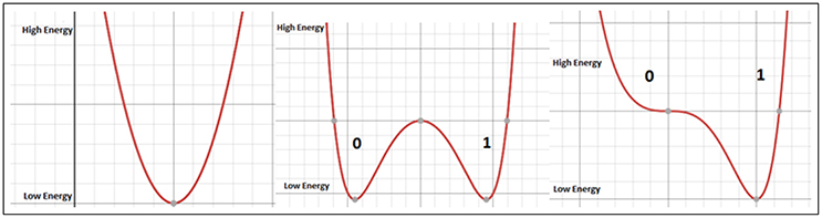
Figure 1. (Left) Initial superposition represented by the minimum energy of the 1-qubit system. (Middle) Double-well potential caused by quantum annealing. (Right) Tilting of the double-well potential by the application of external magnetic fields.

By construction, the qubits always start in the minimum energy configuration. As the problem is introduced, other energy levels get closer to the lowest energy level, which poses a challenge: the smaller the gap between the energy states, the more likely it is that the system will jump from its lowest energy configuration into one of the excited states. The so-called minimum gap is the point where the first excited state approaches the ground state closely, and thermal fluctuations or too short annealing times could result in the system jumping from the ground state to an excited state. If the annealing happens slow enough, meaning that the system stays in the ground state, it follows an adiabatic process. This is particularly worth mentioning, because the larger the system is, the more unlikely it is to remain in the ground state during the annealing cycle.

However, even if the quantum system settles in one of the excited states, this result can be useful. As the system size grows, it becomes harder to classically validate the optimal (minimum energy) solution. Brute force is, for example, classically intractable for even a modest number of qubits (~10⁴). If an excited state is still low-energy enough to be useful in a practical setting, much computation time can be saved by using the quantum annealing system.

Additional built-in devices in D-Wave quantum annealers are the couplers, which allow multi-qubit entanglement. Entanglement refers to correlating qubits in a way that they cannot be described as separate subsystems and act as a single quantum object. Thus, considering a two-qubit system, the change of one qubits state also affects the second qubit, and they can be correlated such that if q₁ ends up in a certain state, q₂ is forced to take the same or opposite state. However, the object q₁q₂ can take 4 different states S = 00, 01, 10, 11, and the relative energy of these states depends on the biases of each qubit, and the coupling between them. This is how a program on the D-Wave quantum annealing system is defined [18]: choosing a set of biases and couplings defines an energy-landscape, whose global minima correspond to the problem being solved. At the end of the quantum algorithm, the system ends up in the minimum energy configuration, thus solving the problem. A classical algorithm would represent the problem in the same way, but where a classical algorithm can walk the surface, the qubits are capable of using quantum tunneling to pass through the energy barriers of the surface. Once entangled, qubits can tunnel together through the energy barriers from one configuration to another. Previous publications have shown how quantum effects in the D-Wave QPU, such as entanglement, superposition, and tunneling, help the QPU solve combinatorial optimization problems [19].

Formalization of the Reinforcement Learning Problem using the Markov Decision Process Framework

The reinforcement learning problem can be described by the Markov decision process (MDP), which consists of states, actions that can be taken in each of these states, state transitions, and a reward function. Furthermore, a distinction between discrete and continuous state spaces, and finite vs. infinite horizon episodes have to be made [20, 21].

States

A set of states S is defined as finite set {s¹, …, s^N}, and each s ∈ S is described by its features, and taking self-driving cars (SDC) as example, some of the features are the SDC's position in the world, other traffic participants (position, velocity, trajectory…), infrastructure (traffic lights, road condition, buildings, construction zones…), weather conditions, …, thus, everything that matters for the SDC in a certain situation at a certain time. Some states are legal, some are illegal, which is based upon the combination of features. It is, for example, illegal for the SDC to occupy space that's occupied by a building or another vehicle at the same time.

Actions

In any given state an agent should be able to evaluate and execute a set of actions, which is defined as the finite set{a¹, …, a^K}, where K characterizes the size of the action space |A| = K. Before we mentioned illegal states, which may result from applying an illegal action for a state, so not every action may be applied in every given state. Generally, we describe the set of actions that may be executed in a particular state s ∈ S by A(s), where A(s) ⊆ A and A(s) = A for all s ∈ S. We also need to account for illegal states, which can be modeled by a precondition function:

$\begin{array}{ll}{f}_{legal}:S\times A\to \left\{true,false\right\}& \left(3\right)\end{array}$

Transition

A transition from a state s ∈ S to a consecutive state s′ ∈ S occurs after the agent executes an action in the former. The transition is usually not encoded in hard rules, but given by a probability distribution over the set of possible transitions (different actions will result in different states). This is encoded into a transition function, which is defined as

$\begin{array}{ll}T:S\times A\times S\to \left[0,1\right]& \left(4\right)\end{array}$

which states that the probability of transitioning to state s' ∈ S after executing A(s) in s ∈ S is T(s, a, s′). For all actions a, all states s, and consecutive states after transition s′, T(s, a, s′) ≥ 0 and T(s, a, s′) ≤ 1, and for all actions a, $\sum _{s^{\prime }}T(s,a,s^{\prime })=1$. Given that the result of an action does not depend on the history (previous states and actions), and depends only on the current state, then it is called Markovian:

$\begin{array}{ll}P(s_{t+1}|s_t,a_t,s_{t-1},a_{t-1})=P\left(s_{t+1}|s_t,a_t\right)=T\left(s_t,a_t,s_{t+1}\right)& \left(5\right)\end{array}$

where t = 1, 2, … are the time steps. In such a system, only the current state s encodes all the information required for making an optimal decision.

Reward

The reward is given by a function for executing an action in a given state, or for being in a given state. Different actions in a state s may result in different rewards, and the respective reward function is either defined as

$\begin{array}{ll}R:S\to ℝ& \left(6\right)\end{array}$

or as

$\begin{array}{ll}R:S\times A\to ℝ& \left(7\right)\end{array}$

or as

$\begin{array}{ll}R:S\times A\times S\to ℝ& \left(8\right)\end{array}$

Equation (6) gives the reward obtained in states, Equation (7) gives rewards for performing actions in certain states, and Equation (8) gives rewards transitions between states.

Finite Horizon, Discrete State Space

We have been focusing on finite horizon and discrete state space games so far, and in games such as the one used to describe the introduced quantum reinforcement learning example, the foundation for finding “good states” and subsequently approximating an optimal policy are observations in the form of completed games (episodes). In Black Jack, a state is given by the player's current sum (12–21), the dealer's one showing card (given by the values 1–10, where 1 is an ace), and whether or not the player holds a usable ace (given by 0 or 1, where 0 is no usable ace). The two actions the player can execute are either to stick (=stop receiving cards), to hit (=receive another card), given by a ∈ {0, 1}. Every episode is composed of multiple state-action pairs, and for each state-action pair a reward value is given. Although the same state-action pairs may occur in different episodes, it is very unlikely that the reward for these in two episodes is the same, as the reward in a state not only depends from the state, but also from the previous states and actions. What we intend to approximate from n complete episodes is the optimal policy under consideration of all states.

Difference Monte Carlo and Quantum-Enhanced Monte-Carlo Policy Evaluation

Monte Carlo methods learn from complete sample returns, which implies that they are defined for episodic tasks only. An update happens after each episode, so learning happens directly from experience. The goal is to learn the optimal policy given some episodes, and the basic idea is to average the returns after a state s was visited. A distinction has to be made about whether the returns for each visit to s in an episode are averaged, or only first-time visits. Each of the approaches converges asymptotically. As for the used game each state occurs only once per episode, first-visit Monte Carlo policy evaluation is described in Algorithm 1:

ALGORITHM 1.

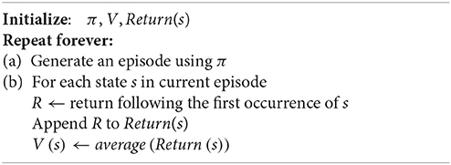
Algorithm 1. Monte Carlo policy evaluation.

where π is the policy to be evaluated, V a state-value function, and Return(s) is initialized as empty list and will hold all s ∈ S. In the Black Jack example, our aim is to have a card sum that is greater than the dealer's sum, but in the same instance we must not exceed 21. A reward of +1 is given for winning the game, 0 reward for a draw game, and −1 for losing the game. The state-value function we approximate is based on the policy α, which is defined as “stick if the sum is 20 or 21, and else hit.” For this, we simulated many Black Jack games using policy α and averaged the returns following each state. Finding the state-value function with a purely classical Monte Carlo algorithm requires thousands of observations (simulations), based on which the returns following each state are averaged (see Figures 2, 3, showing the “no usable ace”-scenario only).

FIGURE 2

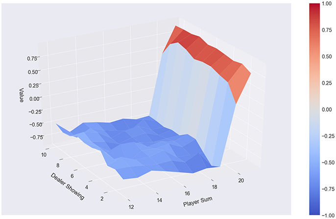
Figure 2. Monte Carlo: 10,000 episodes, policy α, no usable ace.

FIGURE 3

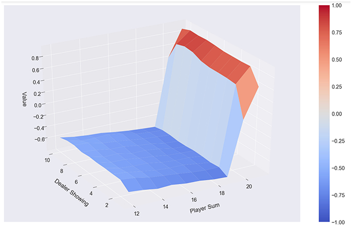
Figure 3. Monte Carlo: 500,000 episodes, policy α, no usable ace.

Additionally, we simulated many blackjack games using random policy β, which would choose a random action in each state, averaged the returns following each state, and used this to find a policy only on observation. The respective value function is plotted in Figure 4.

FIGURE 4

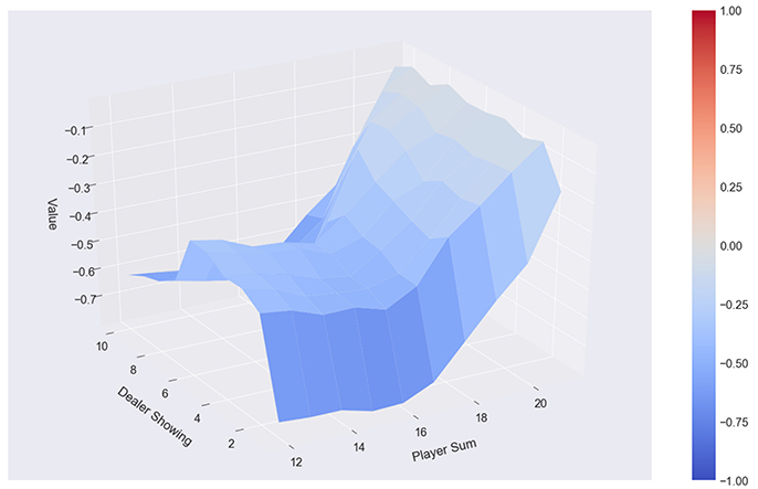
Figure 4. Monte Carlo: 500,000 episodes, policy β, no usable ace.

State-Value Function Approximation

In the first example, we generate n sub-optimal state-value functions by purely classical Monte Carlo policy evaluation. We want to emphasize that the formulation of the algorithm is such that either n classically generated (sub-optimal) state-value functions can be embedded for approximating an improved state-value function, or the state-value functions can be generated quantum-enhanced by supplying episodes with their respective (non-averaged) rewards to the algorithm. Both may also be combined in a nested algorithm. The QUBO formulation is such that it will find the preferable state-action pairs based on their rewards over the episodes, and once this has been completed n times for m episodes, n state-value functions can be generated according to the same proceeding:

• Based on m episodes, find n sub-optimal state-value functions classically and embed each state-action pair with the respective value directly on the QPU and so help to approximate the optimal state-value function, which is better than each of the n sub-optimal state-value functions. How identical state-action pairs over different state-value functions are dealt with will be explained below.

• Based on m episodes, we embed state-action pairs directly on the QPU and approximate a policy directly from the observations.

When using the QPU to approximate the state-value function, we first classically simulated m Black Jack games according to the policy α. We did this n times, and generated n sub-optimal state-value functions. We then embedded these state-value functions on the QPU such that the QPU acts as a filter, which identifies the state-action pairs that do not positively contribute to approximating the optimal state-value function, and removes these from the result. Still, the result may contain identical state-action pairs with different rewards, but those are averaged over. In our experiments, with the help of the QPU we were on average able to filter out $~\frac{1}{2}$ of the state-action-value triples from the initially supplied observations. Due to the partially stochastic nature of the game and the varying episode-length, the number of different state-action-value triples may vary.

Policy Iteration

Concerning policy iteration, we chose random actions in each state, observed the obtained reward, and use this to learn a policy. The proceeding is similar to the latter example, except that we do not start with a given policy, such as α described above, but try to find a policy (what to do in each state) based observations. By applying the QPU-filter to the original data, we show that we are able to learn policies of similar quality as with the purely classical algorithm, although the number of states in the original data can be reduced by up to $\frac{2}{3}$.

Formulation of the Problem as QUBO

The following explanations are based on classically generated, sub-optimal state-value functions, which are embedded on the QPU. The resulting state-value function is compared with single sub-optimal state-value functions, as well as with a state-value function which was obtained by averaging over all sub-optimal state-value functions. The sub-optimal state-value functions in this example were generated using 100–500 (m) episodes each. We varied the number of generated state-value functions n from 2 to 7. Unsurprisingly, we obtained the best results with 500 episodes and 7 sub-optimal state-value functions. Increasing n by 1 or m by 50 did not allow for embedding the problem on the QPU without splitting it into sub-problems. Here, we explain how to use qubits for representing state-action pairs, and how to determine the entries of the QUBO by using the value per state-action pair we obtained in our sub-optimal state-value functions. In a nutshell, we use the 2-dimensional physical architecture of the chip as if it was 3-dimensional by representing the problem as a tensor-like structure, but the introduced method generalizes to more complex problems with n dimensions. Based on the following explanations it will become obvious that the more observations are supplied, the more qubits and connections between single qubits are required. Thus, as we have to deal with sparse connectivity and a limited number of qubits, it is in our interest to find a formulation of the problem that allows us to find a sufficiently good state-value function for a given policy by keeping the number of observations small.

Conditions

What we approximate is a state-value function for a policy based on observations (complete episodes), and the reward that is given for an action in a given state. Certainly, it is not possible to just rely on one observation, as in each episode we can see a certain state-action pair only once, and thus only are given one reward-value. It may be that in one episode a certain action for a certain state is rewarded higher than in another episode, depending on which actions have been executed in which states in the past. Furthermore, a game such as Black Jack features stochastic components, thus we assume it is possible to make some assumptions about future states (i.e., the player's current sum in an ongoing episode will not decrease in the next state), but it cannot be accurately predicted. This means that we should not ignore the future states in a given state completely, but have to include them into our considerations to a certain degree. Therefore, for formulating the problem as a QUBO we need to consider the following conditions:

• As identical state-action pairs may be rewarded differently in different episodes, we must assume that in the worst case the execution of a certain action given a certain state is positively rewarded in one episode, and negatively rewarded in another episode. As we intend to not only identify random successful state-action pairs, but successful sequences (see condition 2), averaging or any other means of aggregating the rewards of state-action pairs is prohibited, and the QUBO must be formulated such identical state action-pairs over the episodes are given different entries.

• As the reward in a certain state partly depends on what happened in the past, and we are dealing with multiple episodes and want to consider the success of an action in a given state by evaluating the future states, the QUBO must be formulated such that both actions taken in past and future states are taken into account, which allows us to not only determine preferable state-action pairs, but preferable state-action chains by indirectly encoding the statistical probability of consecutive state-action pairs being successful or not while approaching the end of the game. If, in our observed episodes, we find state-action-sequences (s′, a′, s″, a″, s‴, a‴ …) and (s*, a*, s**, a**, s***, a*** …), and the latter comes with higher rewards for consecutive state-action pairs, we assume that this is a more successful sequence. If k >> l and a sequence b gives positive reward k times, and negative reward l times, b will be considered as successful sequence, as k times the cumulative positive reward outweighs the l times cumulative negative reward. If for b, only k > l, other successful sequences may outweigh b, and it may not contribute to and appear in the optimal policy. lf for b, k < l or even only k ≈ l then it must not be considered in the resulting optimal policy.

QUBO

Each of the n episodes consists of a different number of states $S_n=\left\{s_1^n,\dots ,s_m^n\right\}$, where m is the number of states in a given episode and may vary over the episodes. For each state $s_x^{n}in{S}_n$ we may also see varying actions and rewards, depending on the history that lead us to $s_x^n$. Furthermore, we may see different actions, depending on whether the player behaved risk-affine or risk-averse in the episode under consideration. Each of the $s_x^n$ must be given a separate entry in the QUBO matrix, as not only the rewards for the state itself, but also the consecutive state-action pairs including their respective rewards may differ. Therefore, the first step is to iterate over all episodes, create a list L of length l containing state-action pairs and the observed negative rewards r*(−1)*r_f in a temporary dictionary, where r_f is a factor applied to scale the reward up or down, depending on the size of the real values. In this given problem, all rewards ranged from (−1) to 1, and we had best successes in scaling up the rewards by a factor of 10. Due to fluctuations during the annealing cycle, the energies of different possible solutions must not be too close to each other, as jumps may happen, i.e., from a lower energy-solution (better) to a higher-energy solution (worse). On the other hand, the higher the energy barriers, the more unlikely tunneling will happen and we may get stuck in a local minimum, so the energy values also must not be too far apart. The negative rewards are needed, as maximizing the reward equals minimizing the negative reward, which can be interpreted as energy minimization problem on the QPU. The basic QUBO-entry for each state-action pair V_{s, a} is thus calculated as shown in Equation (9).

$\begin{array}{ll}{L}_{s,a}=V_{s,a}=R_{s,a}\ast \left(-1\right)\ast r_f& \left(9\right)\end{array}$

The QUBO-matrix is an upper triangular N × N-matrix defined by i ∈ {0, …, N−1} by j ∈ {0, …, N−1}. In the demonstrated example, each entry is first initialized with 0, and subsequently updated with the values of the set $\left\{L_{S,A},L_{S,A}^T\right\}$, where S are all observed states and A the respective actions, obtained from completed games. L_{S, A} is of length n*M, where n is the number of observed episodes and M = {m₀, …, m_n−1} is the number of states per episode, which may vary from episode to episode. If a state-action tuple is given in one episode but missing in others, the entries for the latter remain 0. An entry i, j is updated if a state-action tuple L_{i(s, a)} of an episode is identical to a state-action tuple L_{j(s, a)} of another episode. The entries are given by the following functions (Equations 10–12):

$\begin{array}{ll}QUBO\left(i,j\right)=\{\begin{array}{ll}QUBO\left(i,j\right)+{\left(L_{i\left(v\right)}+L_{j\left(v\right)}\right)}^2,\hfill & ifc1\hfill \\ QUBO\left(i,j\right)-\left({\left(L_{i\left(v\right)}+L_{j\left(v\right)}\right)}^2\right),\hfill & ifc2\hfill \\ QUBO(i,j)\hfill & otherwise\hfill \end{array}& \left(10\right)\end{array}$

where

$\begin{array}{ll}c1:L_{i\left(s,a\right)}=L_{j\left(s,a\right)}and\left(L_{i\left(v\right)}+L_{j\left(v\right)}\right)>0andi\ne j& \left(11\right)\end{array}$

and

$\begin{array}{ll}c2:L_{i\left(s,a\right)}=L_{j\left(s,a\right)}and\left(L_{i\left(v\right)}+L_{j\left(v\right)}\right)<0andi\ne j& \left(12\right)\end{array}$

where L_i(v) gives the ith value v in L_{s, a, v} ∈ L_{S, A, V}, S = {s₁, s₁, …, s_n}, A = {a₁, a₁, …, a_n}. This basically means that we lock each state-action pair in L_{S, A}, and find the respective duplicate state-action pairs over the remaining entries, which are summed and squared to represent the QUBO entries. For this first QUBO manipulation there are several conditions, however, to be considered for writing an entry:

• An entry is only added if it is the summed and squared values are maximum or minimum per L_i(v).

• An entry is only added if the state-action pairs L_{i(s, a)} + L_{j(s, a)} match.

• We intend to find the best action per state given n observations of respective length m_n. As it is most likely that identical state-action pairs appear in different episodes, and as each state-action pair is given a separate QUBO-entry, even if it is identical to one added from another episode, they may not have the same value. We increase or decrease these values quadratically, in order to separate them from one another, which results in a separation or an amplification of identical state-actions based on their values. As we are minimizing energies and therefore multiply the state values by (−1): the smaller $-\left({(L_{i(v)}+L_{j(v)})}^2\right)$ the better.

We add the diagonal terms as follows (Equation 13):

$\begin{array}{ll}QUBO\left(i,j\right)=\{\begin{array}{ll}QUBO\left(i,j\right)+\left(L_{i\left(v\right)}+L_{j\left(v\right)}\right),\hfill & if{L}_{i\left(s,a\right)}=L_{j\left(s,a\right)}andi=j\hfill \\ QUBO(i,j),\hfill & otherwise\hfill \end{array}& \left(13\right)\end{array}$

What follows next is the separation of different state values from one another, as we only want to find the optimal policy, which is the best action in a given state considering the future states. Games like Black Jack have a stochastic component, but nevertheless the history resulting in a state and n observations let us statistically determine what the most likely future states in a given states are. We penalize identical states with different actions as described in Equation (14).

$\begin{array}{ll}QUBO\left(i,j\right)=\{\begin{array}{ll}QUBO\left(i,j\right)+p,\hfill & if{L}_{i\left(s\right)}=L_{j\left(s\right)}and{L}_{i\left(s\right)}\ne L_{j\left(s\right)}andi\ne j\hfill \\ QUBO(i,j),\hfill & otherwise\hfill \end{array}& \left(14\right)\end{array}$

where p is a penalization constant, which should be set to according to the energy scale.

In order to approximate a good policy not only based on high-valued observations, but chains of consecutive states with cumulative high reward, it is possible to consider chains of length h (the horizon) by manipulating the QUBO-entries of h consecutive states. While iterating over all episodes and states, we identify each state s′ following a state-action pair {s, a}, which may differ from episode to episode. For each of the consecutive states s' we create or manipulate the respective entry according to $Equations (15–17).

$\begin{array}{ll}QUBO\left(i,j\right)=\{\begin{array}{ll}QUBO\left(i,j\right)+{\left(L_{i\left(v\right)}+L_{j+k\left(v\right)}\right)}^2,\hfill & ifc1\hfill \\ QUBO\left(i,j\right)-\left({\left(L_{i\left(v\right)}+L_{j+k\left(v\right)}\right)}^2\right),\hfill & ifc2\hfill \\ QUBO(i,j)\hfill & otherwise\hfill \end{array}& \left(15\right)\end{array}$

where

$\begin{array}{ll}c1:L_{i-\left(k-1\right)(s,a)}=L_{j\left(s,a\right)}and\left(L_{i\left(v\right)}+L_{j+k\left(v\right)}\right)>0andi\ne j& \left(16\right)\end{array}$

and

$\begin{array}{ll}c2:L_{i-(k-1)\left(s,a\right)}=L_{j\left(s,a\right)}and\left(L_{i\left(v\right)}+L_{j+k\left(v\right)}\right)<0andi\ne j& \left(17\right)\end{array}$

We initialize k with 1 so that in the first iteration i − (k − 1) = i, and in consecutive iterations i increases with k, and we always consider consecutive states. As identical state-action pairs from different episodes received separate entries, the more often a chain is successful, the more often all of its respective values are increased at different i, j in the matrix. Due to the penalization in Equation (14) different actions per state are already separated. The bigger the horizon, the more qubits we need to represent the problem, and the smaller the original problem must be so that it can be embedded without splitting it into sub-problems.

Experimental Results and Conclusions

By formulating and embedding the QUBO-matrix on the QPU as specified, we are able to show that:

• Given a policy α, which is defined as “stick if the sum is 20 or 21, and else hit,” and a limited number of observations, we can use the QPU as a filter to identify the states or sequences of states that do not positively contribute to approximating the optimal state-value function. We can reduce the source state-action-value triples by up to $\frac{1}{2}$, and by averaging over the remaining values per state, whereby we may still see duplicate state-action pairs in the result, we can generate an improved state-value function. The resulting state-value function, found by the quantum-enhanced Monte Carlo algorithm, is at least equivalent or even better compared to one learned with purely classical Monte Carlo policy evaluation on all given state-action-value triples. Due to the partially stochastic nature of the game and the varying episode-length, the number of different source-state-action-value triples may vary, but here are two examples in support of our explanations: by setting n = 7, m = 500, we obtained 1,072 different state-action-value triples in the source data, with 1,004 of them being distinct. With the QPU-filter, we could reduce the number of state-action-value triples to 618, over which we averaged. In another example, with unchanged n and m, we ran the algorithm five times, and summarized the result to 5,393 state-action-value triples in the source data, with 4,699 of them being distinct. With the QPU-filter, we could reduce the number state-action-value triples to 3,019, over which we averaged. For the latter case, plotted in Figures 6, 7, the Euclidean distance from the state-value function found with the quantum-enhanced algorithm to the optimal state-value function found with the purely classical algorithm and 500,000 episodes (with varying numbers of states) is 2.01, whereas the distance from a state-value function determined with the purely classical algorithm to the (also purely classically determined) optimal policy is 3.26.

• Given a random policy β, in which an action is randomly chosen in each state, and a limited number of observations, we can use the QPU as a filter to identify the states or sequences of states that do not positively contribute to learning a policy which approximates an optimal policy. We can reduce the source state-action-value triples by up to $\frac{2}{3}$, and by conducting a majority vote over the remaining actions per state we can approximate a policy that is equivalent or only slightly poorer than the policy found with the purely classical algorithm on all given state-action-value triples. By setting n = 7, m = 500 and running the algorithm five times and summarizing the result, we obtained 4,904 state-action-value triples in the source data, with 4,489 them being distinct. With the QPU-filter, we could reduce the number state-action-value triples to 1,615. Due to the limited number of observations, we were not able to completely eliminate duplicate states with different actions in the quantum-classical algorithm. Thus, we applied a majority vote, and show that the results produced by the classical algorithm are only slightly better than the ones produced by the quantum-classical algorithm. However, the purely classical algorithm required 4,904 state-action-value triples for making a decision, whereas the quantum-enhanced algorithm was able to filter out 3,289 state-action-value triples and then find a qualitatively similar policy with only 1,615 observations. In the described case, calculating the Euclidean distance from the policy found with the quantum-enhanced to the optimal policy found with the purely classical algorithm and 500,000 episodes (with varying numbers of states) is 10.2, whereas the distance from a policy determined with the purely classical algorithm to the (also purely classically determined) optimal policy is 9.8.

Summing up, we were able to directly embed maximally 7 complete state-value functions generated on 500 observations each on the QPU. With each execution the results slightly vary, which is because of the randomly chosen observations, based on which different numbers of different states-action-value triples are available. We used between 1,100 and 1,700 qubits, a number which also varied with different sets of observations. The considered horizon h can be of arbitrary length, and a discount factor may be used to scale the importance of the future states compared to the actual state, whereby we applied discount factors from 0.1 to 0.9 in our experiments. We were able to show that we can partially formulate policy-evaluation and iteration as QUBO, such that it can be presented to and solved with the support of a D-Wave 2000Q QPU. We were also able to show that by augmenting Monte Carlo policy evaluation, which calculates the value function for a given policy using sampling, with the introduced algorithm, we obtain equivalent or slightly better results compared to averaging over n state-value functions or to each of the sub-optimal state-value functions (with identical m). The state-value functions we found based on the n episodes and sub-optimal state-value functions are still not optimal, compared to classically found state-value functions based on tens or hundreds of thousands of observations. Figure 5 shows the state value function (assuming the player has a usable ace) based on the classical Monte Carlo algorithm. Figure 6 shows the state-value function based learned from averaging over 5 iterations and 7 classically found state-value functions. Figure 7 shows the results produced by the quantum-classical algorithm, which, in this case, produces a better result than the classical algorithms with the same parameters.

FIGURE 5

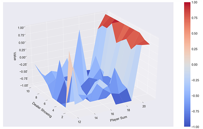
Figure 5. Classical Monte Carlo: 500 episodes, policy α, no usable ace.

FIGURE 6

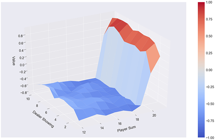
Figure 6. Classical Monte Carlo: 500 episodes, 7 policies, policy α, averaging over results, no usable ace.

FIGURE 7

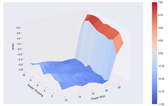
Figure 7. Quantum-enhanced Monte Carlo: 500 episodes, 7 policies, policy α, averaging over results, no usable ace.

Future Work

In this report, we showed how to partially embed policy evaluation for discrete state spaces on the D-Wave QPU, whereas in our current work we aim to find quantum-classical algorithms capable of dealing with continuous state spaces, which is, i.e., ultimately useful in the context self-driving vehicles, where an agent needs to be able to make decisions considering a dynamically changing environment based on continuous state spaces (we must emphasize that due to the very early stage of quantum hardware development, the applicability of this work for SDCs and similarly complex scenarios lies in the distant future). Furthermore, actions cannot necessarily be discretized, i.e., when we consider reinforcement learning in terms of self-learning/healing machines, which we also aim to solve. We will continue to focus on solving practically relevant problems by means of quantum machine learning [22–27], quantum simulation, and quantum optimization.

Author Contributions

FN: research on how to formulate the Monte Carlo Policy iteration as QUBO, code for implementation, writing the publication; DVD: research on how to formulate the Monte Carlo Policy iteration as QUBO; CS and GC: contributions to the code.

Conflict of Interest Statement

The authors declare that the research was conducted in the absence of any commercial or financial relationships that could be construed as a potential conflict of interest.

Acknowledgments

Thanks go to VW Group CIO Martin Hofmann and VW Group Region Americas CIO Abdallah Shanti, who enable our research.

References

1. D-Wave. Quantum Computing, How D-Wave Systems Work (2017). Available online at: https://www.dwavesys.com/quantum-computing

2. Benedetti M, Gmez JR, Biswas R, Perdomo-Ortiz A. Estimation of effective temperatures in quantum annealers for sampling applications: a case study with possible applications in deep learning. Phys Rev A (2015) 94:022308. doi: 10.1103/PhysRevA.94.022308

CrossRef Full Text | Google Scholar

3. Smelyanskiy VN, Venturelli D, Perdomo-Ortiz A, Knysh S, Dykman MI. Quantum annealing via environment-mediated quantum diffusion. Phys Rev Lett. (2015) 118:066802. doi: 10.1103/PhysRevLett.118.066802

PubMed Abstract | CrossRef Full Text | Google Scholar

4. Venturelli D, Marchand DJJ, Rojo G. Quantum annealing implementation of job-shop scheduling. (2015) arXiv:1506.08479v2 [quant-ph]

Google Scholar

5. Jiang Z, Rieffel EG. Non-commuting two-local Hamiltonians for quantum error suppression. Quant Inf Process. (2017) 16:89. doi: 10.1007/s11128-017-1527-9

CrossRef Full Text | Google Scholar

6. Isakov SV, Mazzola G, Smelyanskiy VN, Jiang Z, Boixo S, Neven H, et al. Understanding quantum tunneling through quantum Monte Carlo simulations. Phys Rev Lett. (2015) 117:180402. doi: 10.1103/PhysRevLett.117.180402

PubMed Abstract | CrossRef Full Text | Google Scholar

7. O'Gorman B, Perdomo-Ortiz A, Babbush R, Aspuru-Guzik A, Smelyanskiy V. Bayesian network structure learning using quantum annealing. Eur Phys J Spec Top. (2015) 224:163. doi: 10.1140/epjst/e2015-02349-9

CrossRef Full Text | Google Scholar

8. Rieffel EG, Venturelli D, O'Gorman B, Do MB, Prystay E, Smelyanskiy VN. A case study in programming a quantum annealer for hard operational planning problems. Quantum Inf Process. (2015) 14:1. doi: 10.1007/s11128-014-0892-x

CrossRef Full Text | Google Scholar

9. Venturelli D, Mandr S, Knysh S, O'Gorman B, Biswas R, Smelyanskiy V. Quantum optimization of fully-connected spin glasses. Phys Rev X (2014) 5:031040. doi: 10.1103/PhysRevX.5.031040

CrossRef Full Text | Google Scholar

10. Perdomo-Ortiz A, Fluegemann J, Narasimhan S, Biswas R, Smelyanskiy VN. A quantum annealing approach for fault detection and diagnosis of graph-based systems. Eur Phys J Spec Top. (2015) 224:131. doi: 10.1140/epjst/e2015-02347-y

CrossRef Full Text | Google Scholar

11. Boixo S, Ronnow TF, Isakov SV, Wang Z, Wecker D, Lidar DA. Evidence for quantum annealing with more than one hundred qubits. Nat. Phys. (2014) 10:218–24. doi: 10.1038/nphys2900

CrossRef Full Text | Google Scholar

12. Babbush R, Perdomo-Ortiz A, O'Gorman B, MacReady W, Aspuru-Guzik A. Construction of energy functions for lattice heteropolymer models: efficient encodings for constraint satisfaction programming and quantum annealing advances in chemical physics. (2012) arXiv:1211.3422v2 [quant-ph].

13. Smolin JA, Smith G. Classical signature of quantum annealing Front Phys. (2013) 2:52. doi: 10.3389/fphy.2014.00052

CrossRef Full Text | Google Scholar

14. Perdomo-Ortiz A, Dickson N, Drew-Brook M, Rose G, Aspuru-Guzik A. Finding low-energy conformations of lattice protein models by quantum annealing. Sci Rep. (2012) 2:571. doi: 10.1038/srep00571

PubMed Abstract | CrossRef Full Text | Google Scholar

15. Los Alamos National Laboratory. D-Wave 2X Quantum Computer. (2016) Available online at: http://www.lanl.gov/projects/national-security-education-center/information-sciencetechnology/dwave/

16. Neukart F, Seidel C, Compostella G, Von Dollen D, Yarkoni S, Parney B. Traffic flow optimization using a quantum annealer. Front ICT (2017) 4:29. doi: 10.3389/fict.2017.00029

CrossRef Full Text | Google Scholar

17. Lucas A. Ising formulations of many NP problems. Front Phys. (2014) 2:5. doi: 10.3389/fphy.2014.00005

CrossRef Full Text | Google Scholar

18. Korenkevych D, Xue Y, Bian, Z, Chudak F, MacReady WG, Rolfe J, et al. Benchmarking quantum hardware for training of fully visible Boltzmann machines. (2016) arXiv:1611.04528v1 [quant-ph].

Google Scholar

19. Lanting T, Przybysz AJ, Yu Smirnov A, Spedalieri FM, Amin MH, Berkley AJ, et al. Entanglement in a quantum annealing processor. Phys Rev X (2013) 4:021041. doi: 10.1103/PhysRevX.4.021041

CrossRef Full Text | Google Scholar

20. Wiering M, van Otterlo M (eds). Reinforcement learning and markov decision processes. In Reinforcement Learning. Adaptation, Learning, and Optimization. Vol. 12. Berlin; Heidelberg: Springer (2012). pp. 3–42.

Google Scholar

21. Sutton RS, Barto AG. Reinforcement Learning: An Introduction. Cambridge: MIT Press (1998).

Google Scholar

22. Neukart F, Moraru SM. On quantum computers and artificial neural networks. Signal Process Res. (2013) 2:1–11.

Google Scholar

23. Neukart F, Moraru SM. Operations on quantum physical artificial neural structures. Proc Eng. (2014) 69:1509–17. doi: 10.1016/j.proeng.2014.03.148

CrossRef Full Text | Google Scholar

24. Springer Professional. Volkswagen Trials Quantum Computers. (2017) Available online at: https://www.springerprofessional.de/en/automotive-electronics---software/companies---institutions/volkswagen-trials-quantum-computers/12170146?wtmc$=$offsi.emag.mtz-worldwide.rssnews.-.x

25. Neukart F. Quantum physics and the biological brain. In Reverse Engineering the Mind. AutoUni Schriftenreihe, Vol. 94. Wiesbaden: Springer (2017). pp. 221–229.

Google Scholar

26. Levit A, Crawford D, Ghadermarzy N, Oberoi JS, Zahedinejad, E, Ronagh, P. Free-energy-based reinforcement learning using a quantum processor. (2017) arXiv:1706.00074v1 [cs.LG].

Google Scholar

27. Crawford D, Levit A, Ghadermarzy N, Oberoi JS, Ronagh P. Reinforcement learning using quantum Boltzmann machines. (2016) arXiv:1612.05695 [quant-ph].

Google Scholar