Patterns and Trends in Cetacean Occurrence Revealed by Shorewatch, a Land-Based Citizen Science Program in Scotland (United Kingdom)

Introduction

The Whale and Dolphin Conservation (WDC) Shorewatch program involves trained members of the public in monitoring coastal cetaceans in Scotland (United Kingdom), based on dedicated effort-based “watches” from the coast, following a standardized protocol. Starting in 2005, the Shorewatch program was developed with support from NatureScot (formerly Scottish Natural Heritage) and has already accumulated an important time series of cetacean sightings from all around the Scottish coast, including information not otherwise collected, such as fine-scale data on the use of the coastal environment by cetaceans, behavior, presence of calves, and the occurrence of rare species, as well as spatio-temporal patterns and trends in all of the above. The program aims to improve our knowledge of the coastal cetacean species present, and their distribution and local abundance, as well as determining seasonal and year-to-year trends and spatial patterns in occurrence and abundance, and to promote conservation of cetaceans and their marine habitat.

To date, the Shorewatch program has reported sightings of 18 different coastal cetacean species, i.e., 75% of the 24 species recorded in the waters around Scotland (Parsons et al., 2000; Weir et al., 2001; Reid et al., 2003). All cetacean species are listed under Annex IV of the EU Habitats Directive (Council Directive 92/43/EEC,) as European Protected Species of Community Interest which are in need of strict protection. Furthermore, the two most commonly sighted species along Scottish coasts, harbor porpoise (Phocoena phocoena), and bottlenose dolphin (Tursiops truncatus) (Weir et al., 2001; Reid et al., 2003; Robinson et al., 2007) are protected under Annex II of this directive. This legislation requires establishment of a system to monitor the species and ensure that human activities do not have a significant negative impact on them and, for species listed in Annex II, the designation of special areas of conservation (SACs). In addition, the EU Marine Strategy Framework Directive (MSFD) (Directive 2008/56/EC,) requires implementation of monitoring and management measures to achieve or maintain good environmental status (GES) in relation to 11 descriptors, the first of which is biodiversity. Cetacean abundance, distribution and fisheries bycatch are all considered when assessing GES in relation to descriptor 1. At present (2021), although the United Kingdom has left the EU, the provisions of these Directives remain in force, since the European Union (Withdrawal) Act 2018 brought all existing EU law into United Kingdom law.

The observation points of the Shorewatch program are, as the name suggests, shore-based. Thus, the sampling effort is limited to coastal areas, which are of particular interest for the conservation of cetaceans because it is where most human marine activities are concentrated. Cetacean species inhabiting those areas face a wide range of threats (Avila et al., 2018), most of them anthropogenic, including fisheries bycatch (Read, 2005), ghost gear entanglement (Stelfox et al., 2016), anthropogenic underwater noise (Wright et al., 2007), vessel collisions (Schoeman et al., 2020), habitat degradation and disturbance (Parsons et al., 2000), infectious diseases (Gulland and Hall, 2005), marine debris (Baulch and Perry, 2014), climate change (MacLeod et al., 2005; Moore, 2005; Learmonth et al., 2006), and chemical pollution (Parsons et al., 2000; Hall et al., 2006; Law et al., 2006; Pierce et al., 2008; Murphy et al., 2015; Jepson et al., 2016).

The threats described, together with the requirements of various relevant directives and laws, dictate the need to monitor coastal cetacean species inhabiting Scottish waters. Monitoring of the abundance and distribution of most cetacean populations in European waters under the EU MSFD and Habitats Directive depends on large-scale, synoptic, boat-based and aerial surveys such as the SCANS surveys, of which there have been three to date, carried out in summer at approximately decadal intervals (Hammond et al., 2013, 2017). For resident coastal populations, such as those of bottlenose dolphins, photo-identification surveys are more appropriate (Cheney et al., 2014, 2019; Arso Civil et al., 2019). Local and regional scale surveys–including land-based monitoring (e.g., Hastie et al., 2004; Weir et al., 2007; Bailey et al., 2013; Dolman et al., 2014)–can potentially provide additional evidence about patterns and trends in cetacean distribution and abundance during the periods between large-scale surveys, and at other times of year, assuming that they meet appropriate quality control standards. For example, the Joint Cetacean Protocol (Paxton et al., 2016) proposes, among other recommendations, that the data supplied on effort and sightings must be related by a common code (to ensure that each sighting can be linked to the relevant unit of effort), and both must be geographically and temporally referenced. Thus, even when protocols vary widely, there are approaches which can be used to integrate multiple data sources so as to be able to infer patterns and trends in cetacean distribution and abundance (e.g., Cheney et al., 2013; Virgili et al., 2019; Waggitt et al., 2020; Bouchet et al., 2021).

Relevant characteristics of the Shorewatch protocol include effort-related sightings data, a well-established and standardized methodology, sites all around the Scottish coast and a time series that now exceeds 15 years in length. Nevertheless, it is important to also consider the potential limitations of such data sets. Firstly, and most obviously, observations are spatially limited (to specific sites) and cover only areas adjacent to the coast. In general, there is an issue that such surveys cover only part of the range of a population (or management unit) and, using the Shorewatch data in isolation, it is therefore difficult to distinguish changes in abundance from changes in distribution. Shorewatch covers most of the range of the coastal bottlenose dolphin population in northeast Scotland (Cheney et al., 2014; Arso Civil et al., 2019) and it is thus interesting to compare apparent abundance trends with those obtained using photo-identification studies of this species. Secondly, although there is year-round search effort (unlike the large-scale surveys), it tends to be irregularly distributed in space and time, and the large numbers of observations taken at particular locations may not be statistically independent of each other. This is likely to be especially true for resident populations, like that of the bottlenose dolphin (Bailey et al., 2013). Thirdly, despite increasing use of citizen science data on cetacean distribution and abundance (Bouchet et al., 2021), there is some skepticism about the use of such data in statutory population status assessments, due to perceived quality control issues such as the use of observers with various levels of training, possible misidentifications, and unconscious bias in effort toward times and locations with high cetacean occurrence.

Previous surveys of the distribution and occurrence of Scottish coastal cetaceans include the aforementioned SCANS surveys, opportunistic data collection during seabird surveys by Seabirds at Sea Team (SAST) and European Seabirds at Sea (ESAS) (Weir et al., 2001; Virgili et al., 2019; Waggitt et al., 2020), and data collected by dedicated volunteer networks (such as SeaWatch and Shorewatch) from opportunistic platforms. Most of the above-mentioned datasets have limited temporal or spatial coverage and for that reason, there remains a need to improve our knowledge about patterns and trends in the occurrence and the use of Scottish coastal waters by cetaceans, not only to meet statutory requirements for monitoring but also to inform the development and implementation of effective management measures against potential anthropogenic threats.

The suitability of Shorewatch data to detect trends in occurrence of bottlenose dolphins in the Moray Firth SAC was previously investigated by Embling et al. (2015). The study concluded that around five watches per day were required to detect year-to-year or between-site differences of 50% in dolphin occurrence, in locations where dolphins were sighted reliably (at least 0.1 sightings per hour), and that differences of less than 30% could not be detected statistically. Here we aim to further explore the suitability of the Shorewatch data to answer various monitoring questions about occupancy and local abundance of cetaceans, and the patterns and trends in space and time that can be detected over different time-scales.

We may expect the presence and local abundance of cetaceans to show temporal variation, and perhaps cycles, at several time-scales (Bailey et al., 2013). The shortest relevant time-scale is linked to the duration of periods that individual animals spend at the surface and underwater. The next relevant time-scale is likely to be sub-daily, for example feeding movements related to the tidal cycle (e.g., Mendes et al., 2002). At longer time-scales, seasonal shifts in distribution may be seen. These patterns will differ between species. For monitoring purposes, the shortest cycles, related to surfacing intervals, may be useful in terms of describing behavior and identifying whether animals are foraging, traveling, resting, engaged in courtship, aggressive interactions or nursing. From a statistical point of view, we wish to obtain accurate and precise measures of presence (or occupancy) and abundance while assuring as far as possible that observations are independent of each other, i.e., eliminating spatio-temporal autocorrelation and thus avoiding pseudo-replication. If successive watches are recording exactly the same individuals, arguably this is a problem because we would be over-estimating the numbers of animals and sightings although, if we are observing animals from a resident population, it is also not surprising, as is the case for resident bottlenose dolphins that may stay in the same area for hours (Hastie et al., 2004; Bailey et al., 2013). Considering all the possible time-scales, the selection of an appropriate duration for the watches is complicated, perhaps more so in programs like Shorewatch, that involve citizen volunteers, in which their interests (e.g., time constraints, the quality of the experience) must also be taken into account. Thus, there is a tension between building a reliable picture of what is happening, obtaining observations which are independent of each other, and ensuring that observers are fully engaged and motivated to continue contributing data.

In this study, the Shorewatch program dataset was analyzed to:

(1) Describe the coverage achieved to date by Shorewatch, in terms of spatial and temporal distribution of the watches. Based on this initial exploratory analysis, we selected seven sites to use for the majority of the further analysis, taking into consideration the number of watches carried out at each site, the length of the time series and the coverage for different times of year.

(2) Evaluate the utility of the dataset to describe cetacean distribution, occupancy and abundance, and its power to describe patterns and detect trends (e.g., between years, seasons and sites), and thus to evaluate the suitability of the Shorewatch program as an effective monitoring tool. We considered evidence about the consistency of species identification, the statistical properties of the data (e.g., existence of autocorrelation) and the precision of the estimates of probability of occurrence and sighting rate. This analysis, coupled with statistical simulations, aims to evaluate the power of the methodology to detect trends and therefore determine its suitability for assessing GES under the MSFD and detecting possible human impacts on coastal cetaceans at a fine scale along the Scottish coastline.

(3) Describe and quantify spatio-temporal patterns and trends in the local occurrence and relative abundance of Scottish coastal cetaceans and to describe the influence of environmental variables. We undertook statistical modeling of the patterns and trends in the local occurrence and relative abundance of the five most frequently sighted species: bottlenose dolphin, harbor porpoise, minke whale (Balaenoptera acutorostrata), Risso’s dolphin (Grampus griseus), and common dolphin (Delphinus delphis).

Materials and Methods

Study Area and Data Collection

The Shorewatch program started in 2005, based at the Scottish Dolphin Centre in Spey Bay (Moray Firth) and was later extended to other land-based observation platforms along the Scottish coastline, mainly from headlands and other vantage points. For the present analysis, data collected between March 2005 and April 2018 were available. At the time of the analysis, the Shorewatch program was operating at 25 locations around the coastline (Figure 1). The features considered when choosing the observation sites include viewing potential (height, field of view); achieving a geographical spread; monitoring potential (history of cetacean sightings); volunteer requirements (proximity, accessibility, and facilities); and support and outreach (local partner support, education and awareness-raising).

FIGURE 1

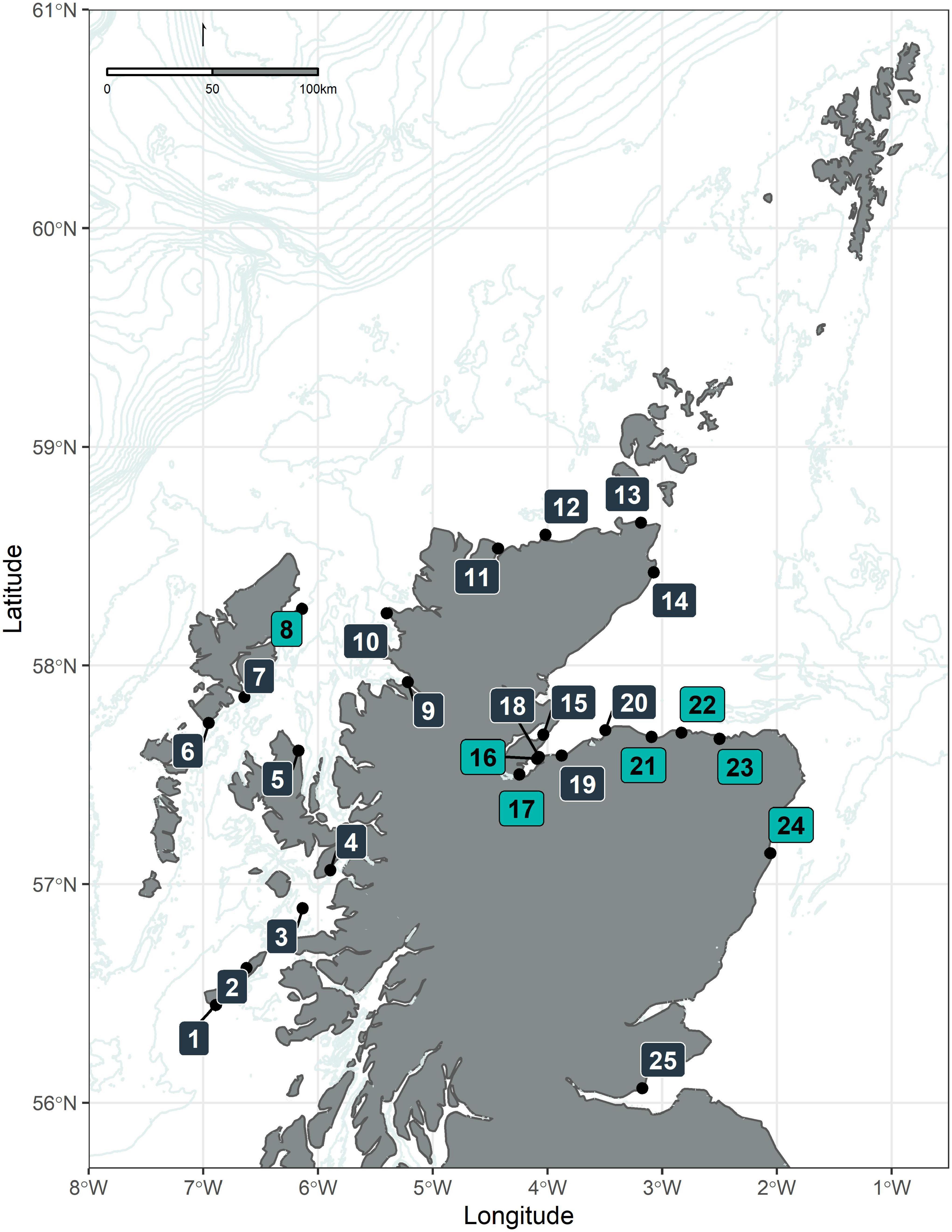
Figure 1. Map of the study area. The map describes the position of the observation sites of the Whale and Dolphin Conservation Shorewatch program: (1) Hynish Watch Tower (Tiree); (2) Hough Bay (Coll); (3) Eigg Pier (Eigg); (4) Armadale Pier (Skye); (5) Kilt Rock (Skye); (6) Rodel (Harris); (7) Scalpay Lighthouse (Harris); (8) Tiumpan Head (Lewis); (9) Rhue Lighthouse (Ullapool); (10) Stoer Head Lighthouse; (11) Melness Church (Talmine); (12) Strathy Point; (13) St John’s Point (Caithness); (14) Castle of Old Wick; (15) Cromarty; (16) Chanonry Point; (17) North Kessock; (18) Fort George; (19) Nairn viewpoint; (20) Burghead; (21) Spey Bay (Scottish Dolphin Centre); (22) Cullen; (23) Macduff; (24) Torry Battery (Aberdeen); (25) Kinghorn (Fife). Observation sites colored in light blue indicate those locations used for further analysis in this study.

Since the beginning of the program, dedicated visual surveys for cetaceans have been carried out by trained volunteers following a standardized protocol. The effort unit in the protocol is a watch, a period of observation that lasts for 10 min. Watches may be carried out a maximum of once per hour at a given site, i.e., the start times of consecutive watches must be separated by 60 min. Observers use 7 × 50 binoculars with reticules and the naked eye to scan the area. In principle, watches take place at sea states varying between 0 and 4 on the Beaufort scale and under good visibility conditions [visibility is estimated on a scale from poor (range of visibility between 1 and 5 km) to excellent (range of visibility up to at least 20 km)], which facilitates detection of animals and makes occurrence data more reliable. Nonetheless, a small percentage of watches (0.04%) took place in less favorable conditions.

When a watch starts, information is recorded about the date, time, location, and environmental conditions (sea state and visibility), as well as the presence of feeding seabirds and human activities. When cetaceans are sighted, the species is recorded along with a code to describe the observer’s level of confidence in the identification, the numbers of adults and calves seen, their behavior, the estimated distance of the sighting from the observation point and the times (within the watch period) when the sighting started and ended. The end time of the watch is also recorded and each watch is assigned an identification code.

Data Analysis

Exploration of the Data

The dataset was explored to determine the species seen most frequently, to identify the observation sites and time periods with most data available for subsequent analysis, and to describe and visualize the spatial and temporal distributions of observation effort and sightings.

Observation sites are located along the Scottish coastline, irregularly distributed and, in certain cases, they present peculiarities that could lead to overestimation of the number of sightings. In particular there were (i) pairs of sites for which the fields of view overlapped (e.g., Chanonry Point and Fort George) and (ii) sites where the field of view is wider than 180° (e.g., Tiumpan Head and Burghead) and, since a single watch cannot effectively cover such a wide viewing angle (the estimated binocular field of view in humans is 120°), they are split into two consecutive survey areas for which the data are entered separately (e.g., as Tiumpan Head A and Tiumpan Head B). Such sites were merged for analysis. Where observation periods overlapped, one set of observation was removed. In addition, the exact watch point at some sites has been relocated within the local area. Such pairs of sites were also joined to create single time series (e.g., Stoer Head and Nairn).

The data are potentially prone to temporal autocorrelation. Within-day temporal autocorrelation (i.e., between successive watches at a site) is difficult to evaluate directly since each time series consists of a maximum of 8–10 data points (often fewer). However, an indication of the within-day temporal autocorrelation was provided by calculating the overall correlation (across sites and days) between the results from each watch and (if there was one) the following consecutive watch at the same site on the same date (i.e., autocorrelation at lag 1 h). Similar calculations were carried out for lags of 2 h, 3 h, and so on, where the time series at a particular site on a particular day was long enough to permit its inclusion (sample size inevitably declines for longer time lags).

To remove the apparent temporal autocorrelation within the same day in subsequent statistical analysis, watches were aggregated by site and date (see below). For each site-date combination, mean values (across all watches) of the response and explanatory variables were calculated.

Temporal autocorrelation between watches from consecutive days at the same observation site was investigated using site-date aggregated data. The frequency of occurrence of different length runs of observation days was first calculated and plotted. Then, the overall correlation between the results from each day and its following days, at the same site, was calculated.

Data Subsetting

For the present analysis, all watches performed at sea state of 4 or lower and with good visibility conditions (visibility from 1 to >20 km) were used, thus retaining 99.96% of the data. The percentage of watches associated with cetacean presence fell slightly due to this subsetting, from 22.0 to 21.7%. Only those sightings with an associated identification certainty of 100% were used in further analysis. This resulted in the loss of 5.53% of sightings of the five most commonly sighted species (bottlenose dolphin, harbor porpoise, minke whale, Risso’s dolphin, and common dolphin).

Two subsets were then created for use in specific analyses. Subset A includes effort data for those site-date combinations where at least 10 consecutive watches were carried out at a site on a single day (N = 861 site-date combinations). The unit of this subset is the individual watch. Due to the number of daylight hours required to perform 10 consecutive watches in a day, this subset contains data collected from March to October.

Subset B includes effort data for sites with good seasonal coverage (at least 20 watches in each month of the year) over at least 6 years. Only seven observation sites met these criteria between 2012 and 2017 (coverage prior to 2012 was less complete): Tiumpan Head, Chanonry Point, North Kessock, Spey Bay (Scottish Dolphin Centre), Cullen, Macduff, and Torry Battery (Aberdeen). The resulting subset contained 29032 watches (55.11% of the total) that were combined into 8836 unique site-date combinations. As noted above, the use of site-date as the unit for this subset will allow us to eliminate the possible temporal autocorrelation within the same day in further analysis. The topographical characteristics of the observation sites selected (e.g., height) vary according their geographic location. More information can be found in Supplementary Table 1.

Comparisons of Data From Consecutive Watches

Using Subset A, we investigated: (1) variation in sighting rate over consecutive watches, to check whether there is evidence that observer behavior changes over successive watches; (2) differences in sighting rates for watches which were and were not followed by another watch immediately afterward, to check whether successful watches encourage observers to carry out further watches; (3) whether sighting rate for a watch was related to the number of consecutive watches which followed, again to check for evidence that the motivation of observers depended on the results of the watches; (4) variation of cumulative sighting rate over consecutive watches and its variance, to determine how rapidly the estimated sighting rate stabilizes and how variance changes as further watches are carried out.

It should be noted that observations at a given site on a given day are not necessarily all carried out by a single observer. The number of volunteers per day varied between observation sites, with a median of two and a maximum of six volunteers per day in Spey Bay, a median of one and a maximum of three volunteers per day in North Kessock, and a median and maximum of one volunteer per day in Macduff. Thus, whether a second watch took place after the first, and so on, is not necessarily a decision taken by a single person. Furthermore, where multiple individuals are present, individual observers may join the group or leave the group during the sequence of watches.

Ability to Detect Changes in Sighting Rates

In order to set a minimum level of observation effort required to permit detection of trends in local abundance of coastal cetacean populations, we used the IUCN criterion for abundance changes which would identify a population as vulnerable. This criterion has also been proposed [by the ICES Working Group on Marine Mammal Ecology (WGMME), see ICES (2014)] as a basis for determining GES under the MSFD. This approach suggests that population sizes should be maintained at or above baseline levels, with no decrease from this level of more than (or equivalent to) 30% over a three-generation period. Generation times were derived from the literature and the percentage of decrease per year that would be equivalent to a 30% of decrease over three generations was calculated for the main coastal cetacean species present in Scotland (Table 1). According to Article 17(2) of the EU MSFD, Member States (MS) have to update their marine strategies every 6 years. In addition, the EU Habitats Directive has a 6-yearly reporting interval and we thus considered the use of annual data from a 6-year period [i.e., a series of seven annual abundance index (sighting rate) estimates] as appropriate to detect trends in cetacean abundance.

TABLE 1

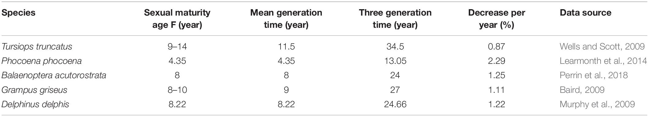
Table 1. Generation time and decrease per year that should be detected for the main coastal cetacean species present in Scotland, calculated based on a 30% decrease over three generations.

Taking into account this information, simulations can be made to calculate the effort necessary to detect a decline with a given statistical power and/or to detect a certain rate of decline. ICES WGMME proposed a minimum power of 80% (see ICES, 2014, 2016), given different underlying levels of decline over a 6-year period. We also considered 95% power. In both cases we assume that a statistically significant trend is one for which p < 0.05 (although this too could be modified). The parameters necessary to perform the simulations are: initial probability of sighting each species (i.e., the initial sighting rate), maximum number of watches that can be carried out (taking into account the number of daylight hours available), the period of time (e.g., 6 years) and the different levels of decline that we want to test. The range of sighting rates chosen corresponds to values obtained in this study for the main cetacean species sighted. In principle, the approach can be easily extended to populations or areas with lower or higher sighting rates.

In the first set of simulations, it was assumed that data would be collected over the whole year at one site, giving an upper limit for the number of watches of ≈4000 (considering average daylight hours over the year). In addition, it was assumed that each watch is a valid and independent estimate of the underlying sighting rate (thus ignoring the issue of autocorrelation). Nonetheless, considering more than one site in future simulations is recommended since spreading out the watches not only over the year but also over several sites could help to ensure independence (ICES, 2014, 2016). The power to detect trends was set at the 80 and 95% level. Since the proportion of watches with more than one sighting is low (3%), it is reasonable to assume a Bernoulli (i.e., 0, 1) distribution of sightings per watch.

Simulations to detect a decline, with a given statistical power, were performed as follows:

(1) For each possible combination of sighting rate and rate of decline per year, generate a sample of X watches (each with a sighting rate of 0 or 1), X being the number of watches which are carried out in a year (from 10 to 4010, in steps of 10) at a site, from a Bernoulli distribution with an appropriate mean value of sighting rate (for the species and site chosen). This provides results for year 0.

(2) For years 1–6, the process is repeated, but each year the underlying sighting rate is reduced by an amount sufficient to achieve the desired overall rate of decline after 6 years.

(3) For each sample size between 10 and 4010, fit a linear regression using year as a covariate to the seven values obtained and check if a trend is detected (regression slope significantly different from 0, at the 95% level, over the 6-year period).

(4) Resample and repeat the calculations 1000 times for each combination of initial sighting rate and rate of decline per year.

(5) Summarize the results of the simulations for each possible combination of initial sighting rate and proportion of decline to be detected over a 6-year period, identifying how many samples are needed to achieve statistical significance 80 or 95% of the time.

The above approach focuses on detecting a statistically significant decline. In the second set of simulations, we determined the number of watches in a year required to detect a particular rate of decline, given a tolerance limit, 80 or 95% of the time. The tolerance limits considered were: 1, 5, 10, 20, 30, and 40%. Steps 1, 2, and 4 are identical to the previous approach. The calculations carried out at steps 3 and 5 are different.

At step 3, for each sample size between 10 and 4010, fit a linear regression using year as a covariate to the seven values obtained and collect the value of the simulated regression slope. For each simulated regression slope check whether it is above or below the lower interval defined by the true regression slope (for the relevant initial sighting rate-rate of decline combination) and the tolerance limit. Thus if the true slope was −2.0 and the tolerance limit was 10%, the relevant rate of decline is considered to have been detected if the simulated slope is negative with a slope equal to or steeper than −1.8. These calculations are repeated for all chosen tolerance limits.

At step 5, summarize the results for each possible combination of initial sighting rate and proportion of decline to be detected over a 6-year period, given each tolerance limit, identifying how many samples are needed to detect this rate of decline 80 or 95% of the time.

Modeling Patterns and Trends in Cetacean Sightings

To investigate the influence of environmental conditions on coastal cetacean occurrence, generalized additive models (GAMs) were used, as they can be used for response variables with different distributions and account for non-linear effects of multiple explanatory variables, while being readily adaptable to fit simple relationships if non-linearity is not apparent (Hastie and Tibshirani, 1990; Wood, 2006, 2017). Subset B was used for fitting the models: this comprises site-date data for seven sites. Modeling was focused on the five most commonly sighted species: bottlenose dolphin, harbor porpoise, minke whale, Risso’s dolphin and common dolphin.

Five response variables were considered in the models for each of the cetacean species selected: (1) occurrence (presence-absence); (2) the number of sightings (total number of sightings per site-date unit); (3) group size (mean group size per site-date unit, rounded up to its nearest whole number); (4) total number of animals sighted (per site-date unit); and (5) mean number of animals (mean number of animals per watch). Several distribution families were tested to identify the best for response variables 2–5, through the evaluation of model diagnostics and predictive performance [similar to the approach used in Potts and Elith (2006)]. Given the nature of the variables, binomial distribution is assumed for variable 1 and Poisson, quasi-Poisson or negative binomial are potentially suitable for variables 2 and 4 (which are count based). However, variables 3 and 5 are daily mean values, resulting in non-integer data, for which quasi-Poisson or negative binomial are the candidates. The use of mean values for each site-date unit basically scales the absolute values of each response variable downward to the values expected in a single watch.

Information collected during the watches about observation time, location and environmental conditions provides several explanatory variables for the models, namely: site (as an ordinal variable, numbering the sites from west to east), latitude-longitude (included in the models as two separate smooth terms), start time of the watch (24 h format), date, visibility and sea state, among others (Table 2). The daily mean values of these variables collected during the watches were calculated for each observation site. We also investigated the apparent influence of several other static and dynamic environmental variables known to affect cetacean distribution (see Table 3). The value of the dynamic environmental variables, derived from remote sensing, for each site-date unit were calculated as the daily mean of those satellite data points that fall within the field of observation of each observation site. On the other hand, the mean value of the static environmental variables (e.g., depth or angle of slope) were calculated for each site taking into consideration all values in the field of observation. Environmental covariates were selected based on their known influence on cetacean distribution directly or through their influence on prey abundance (Bailey and Thompson, 2010; Anderwald et al., 2012; de Boer et al., 2014; Cox et al., 2018). It should be noted that the static variables will have a single value per site.

TABLE 2

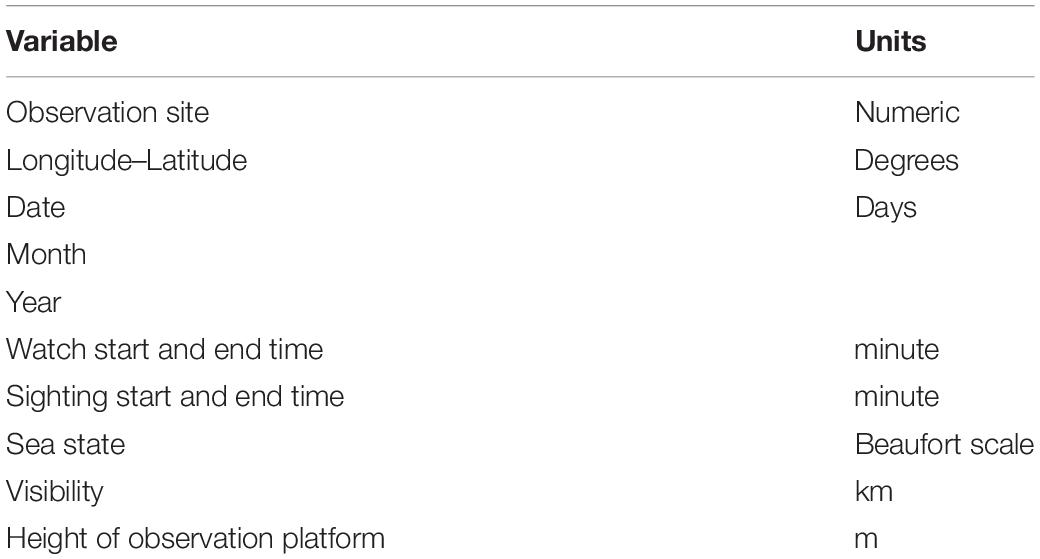
Table 2. Spatio-temporal and other explanatory variables recorded during the watches.

TABLE 3

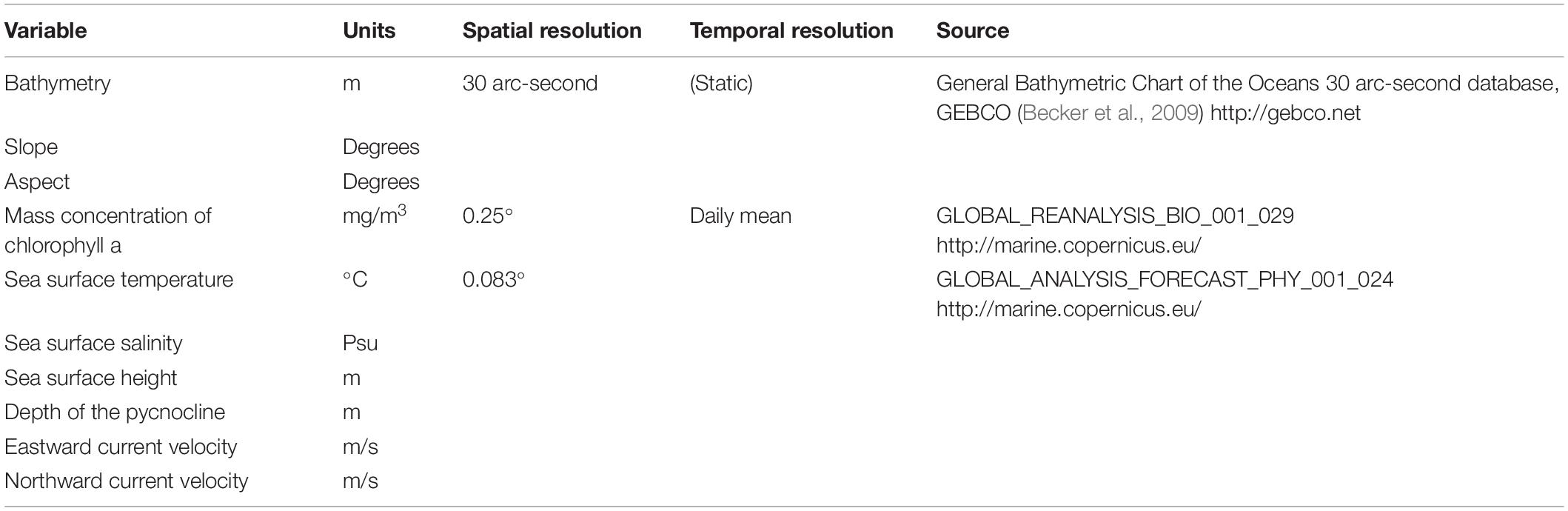
Table 3. Environmental variables, derived from remote sensing, included in the models.

Although tidal state and tide height are potentially useful as explanatory variables for some cetacean species in coastal areas, such as harbor porpoise (Waggitt et al., 2018) and bottlenose dolphin (Mendes et al., 2002), they have not been included in the models because using site-date as the unit means that sub-daily temporal variation is largely obscured (and the set of watches at a site over the course of a day may well span an entire tidal cycle).

To avoid collinearity between explanatory variables, pairwise Spearman correlation coefficients (ρ) were calculated before fitting the models for each species. In the case of highly correlated variables (ρ > | 0.7|) (Dormann et al., 2013), they were added separately to the models and the variable with greater influence on the response variable was selected. Concurvity tests were also performed after fitting the models to avoid unstable estimates, among other problems (Wood, 2008).

Model fitting was carried out using backward selection, starting from saturated models, containing all possible explanatory variables (noting that only one variable from any highly correlated pair can be included), and eliminating non-significant terms one at a time, starting with the least important in the model. If eliminating a variable resulted in no significant reduction in goodness of fit (based on the AIC for the binomial models and ANOVA for the rest of the models), the simpler model was preferred, following the principle of parsimony, and the process was repeated until no more variables could be removed. Note that we did not consider interactions between explanatory variables since there was no strong evidence of such interactions being present.

The maximum number of splines for smoothers was set to four to avoid overfitting (Lambert et al., 2017), except for the covariate month for which was set to 12. The covariates aspect and month were modeled using cyclic smoothers to account for their circular nature. Goodness of fit of the final models was evaluated based on the REML score, deviance explained and correlation between observed and predicted values, as well as by confirming an absence of (i) important trends or patterns in residuals (in general and versus each explanatory variable), (ii) influential data points, (iii) concurvity, and (iv) substantial over- or under-dispersion. Once the best model was selected, predicted values and their standard errors were calculated for each response variable, based on the mean observed conditions at the time and place of each observation.

To investigate the possible effect of autocorrelation across consecutive days on model results, GAMMs were fitted with an AR(1) structure, which assumes that autocorrelation exists only between consecutive days and not over a longer time-scale (e.g., Hastie and Tibshirani, 1990; Wood, 2006; Wood et al., 2015), using Subset B, for which the unit is the site-date, to fit the models. While more complex AR models might be appropriate (to account for autocorrelation over a longer time-scale), because the data comprise a large number of short time-series, we considered this to be impractical.

As an alternative GAMM approach to address temporal autocorrelation at larger scales, considering data from each observation site as independent of data from other sites but allowing that temporal autocorrelation could span a whole month, months were labeled with a unique ID, in chronological order, over the entire study period, then creating the variable site-month, so that each site-month combination has a unique ID. Site-month was then included in the models as a random effect. Since within-day autocorrelation is not an issue when using this structure, we used the original dataset in which the unit for the response variable is the individual watch, rather than the site-date dataset. We chose to focus on the occurrence of the five most frequently sighted cetacean species (separately), as response variables. Explanatory variables were the same as used previously.

Data exploration and analysis were performed using R software (R version 4.0.3) (R Core Team, 2020). GAMs and GAMMs were fitted using mgcv library (Wood, 2017), and figures were produced using the package ggplot2 (Wickham, 2016).

Results

Data Exploration

Effort

From March 2005 to April 2018, 52677 watches were carried out, giving a total of 8779.5 h of effort, i.e., the equivalent of almost 1 year of continuous observation (if all hours were daylight hours). While most observation effort occurred between April and October, over the 13-years study period, cumulative totals of at least 2000 watches have been logged in every calendar month. Effort was highest between 10.00 and 16.00 h and there were few observations earlier than 07.00 h or later than 21.00 h. Evidently, there was also seasonal variation in watch times as daylight hours change over the year. Most watches took place at sea states between 1 and 3 and at high visibility (Figure 2).

FIGURE 2

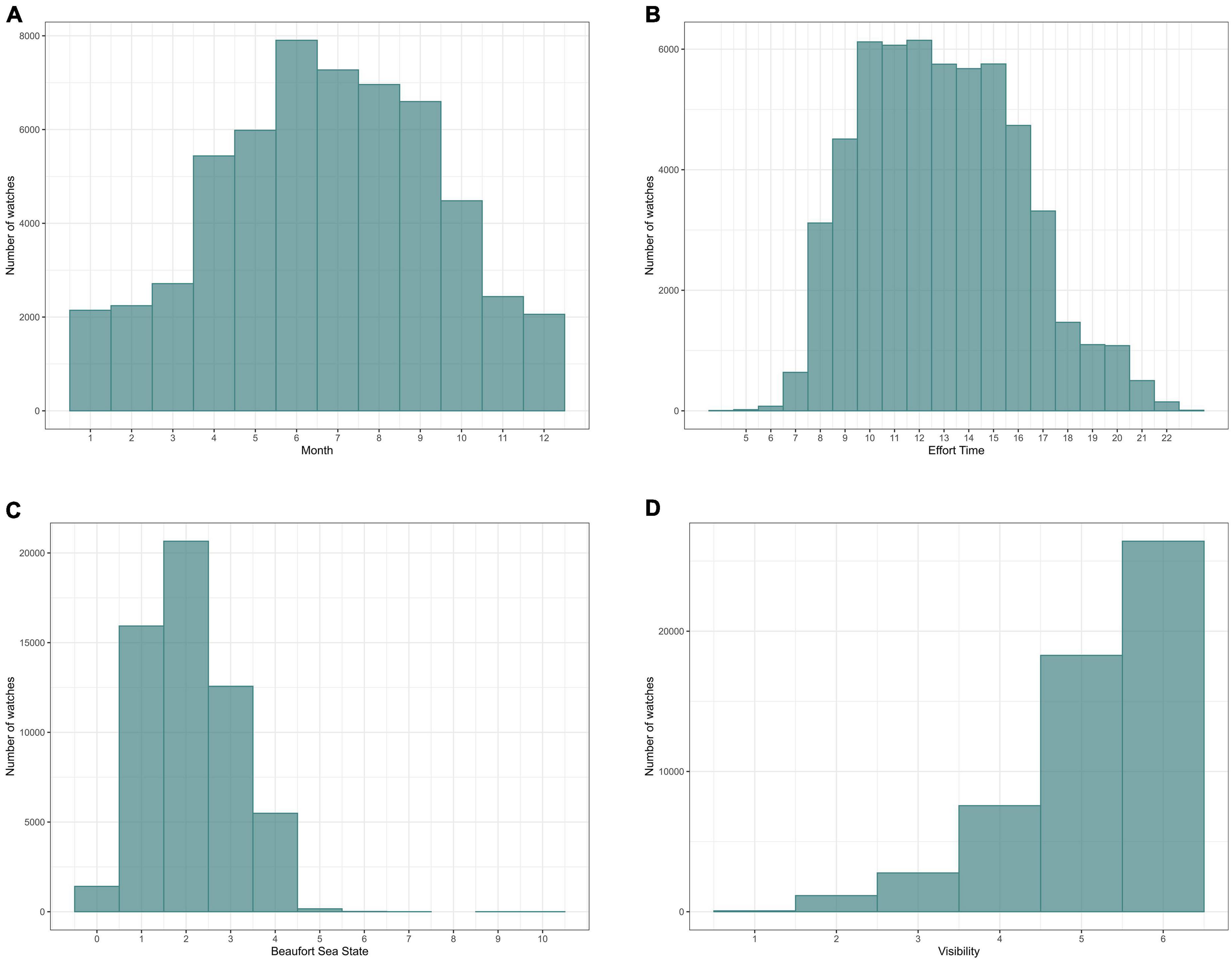
Figure 2. Effort distribution in relation to (A) month; (B) time of day; (C) (Beaufort) sea state and (D) visibility. The y-axis indicates the total number of watches.

Due to the way the Shorewatch program evolved, with new observation sites being added and some discontinued, there was considerable variation in the length of time series for different sites and in the total number of watches per year (Supplementary Figure 1). The longest time series is that for Spey Bay (2005–2018), where the WDC Scottish Dolphin Centre is located and where the Shorewatch program started. Other locations with moderately long time series (7–9 years) are: Chanonry Point, Cullen, Macduff, North Kessock, Tiumpan Head, Torry Battery (Aberdeen), and Nairn (Figure 1). By contrast, there are several sites for which the time series are as short as 1 year, either because they have been added recently or because they have been trialed and rejected for various reasons (e.g., not appropriate for volunteers or insufficient data were being collected). Effort intensity also varied widely across observation sites. There were over 1500 watches on average per year at Spey Bay and a further 13 sites had more than 100 watches per year.

Sightings

Eighteen different cetacean species have been recorded by Shorewatch program. Of these, the five most frequently sighted are bottlenose dolphin, harbor porpoise, minke whale, Risso’s dolphin, and common dolphin (Table 4). The total number of cetacean sightings varied markedly between different observation sites and from month-to-month, although these distributions are strongly influenced by the distribution of search effort (Figure 3). Each species presents a significantly different mean group size (Kruskal-Wallis chi-sq = 1639.9 (p < 0.05); p < 0.05 for all the pairwise comparisons between species), ranging from 1 individual for minke whale up to groups of 12 individuals for common dolphin (Table 5).

TABLE 4

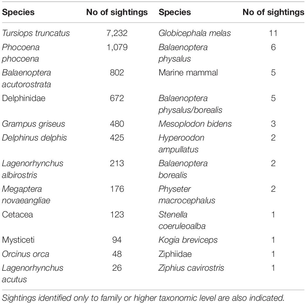
Table 4. Number of sightings per species.

FIGURE 3

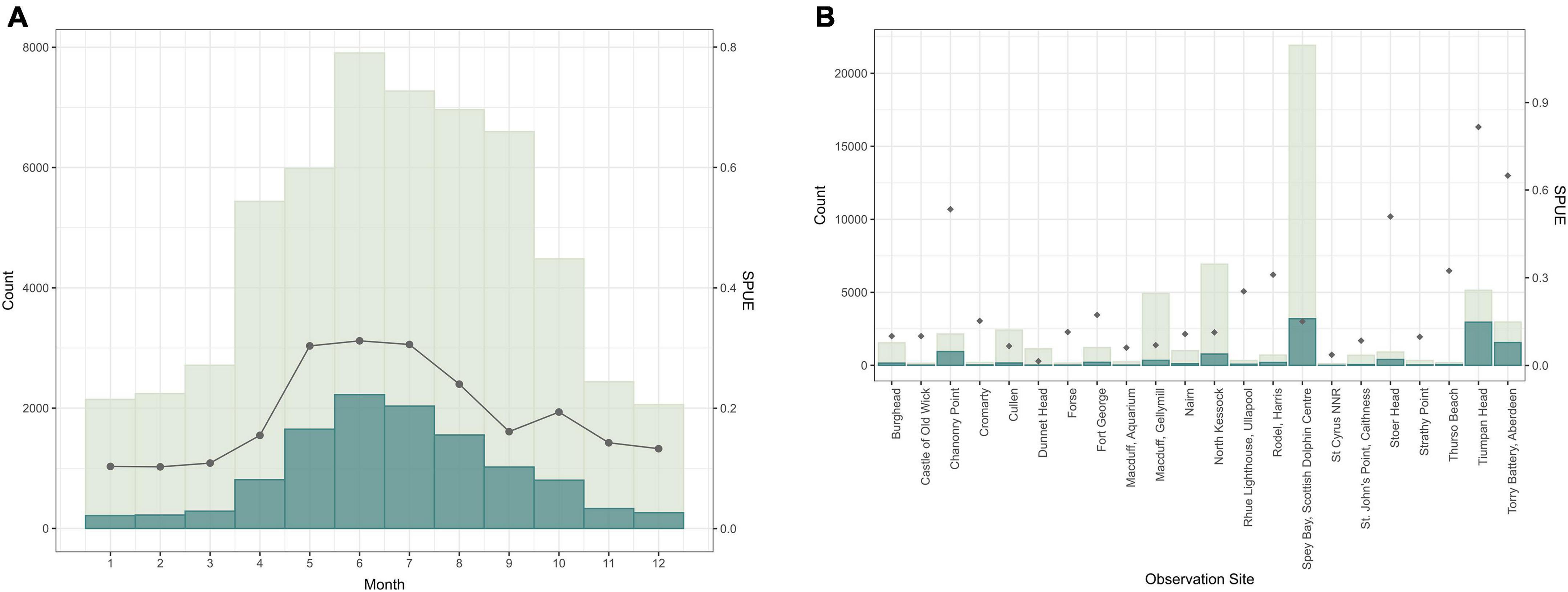
Figure 3. Number of sightings of all the cetacean species for those observation sites with more than 100 watches in relation to (A) month and (B) observation site (scaled on the left y-axis). The number of sightings is shown in dark blue and the distribution of total effort (number of watches) is shown in light gray. Sightings per unit of effort (SPUE) are indicated by dark gray dots, scaled on the right y-axis.

TABLE 5

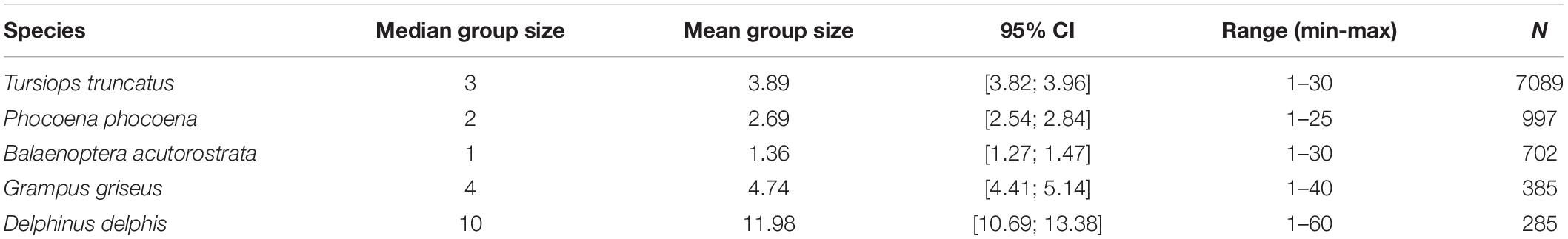
Table 5. Mean group size and its 95% confidence intervals calculated via bootstrapping, minimum and maximum number of individuals in a group and sample size used for the five most sighted species.

Autocorrelation

Correlation analysis, run using Subset A which contains effort data for those site-date combinations where at least 10 consecutive watches were carried out at a site on a single day (these data are consequently all from March to October), showed that sighting rates (for all cetacean species combined) from consecutive watches tend to be moderately correlated (r < | 0.51|). There was also significant temporal autocorrelation between sighting rates for pairs of watches that occurred 2 h apart. This could indicate that some animals stay in the area over several hours so that when consecutive watches are performed, the same animals or groups are counted.

When analyzing the correlation between the sighting rate of consecutive watches separately for each species, the results showed that bottlenose dolphin sighting rates (N = 1197) are moderately correlated (r < | 0.56|) and that statistically significant correlation extends to time-lags of 3 or 4 h. For the rest of the species, there were not enough occurrence data in Subset A to extract correlation values [e.g., harbor porpoise (N = 30) or common dolphin (N = 3)].

The frequency distribution for the length of runs of consecutive days of observation at a given site showed that most site-days were either isolated (with no observations on the previous or subsequent days at that site) (40%) or belonged to a short run of consecutive observation days (2–3 days = 29%) at a site (Figure 4). Very long runs of consecutive observation days are the exception, 276 days being the maximum run length (observations carried out at North Kessock).

FIGURE 4

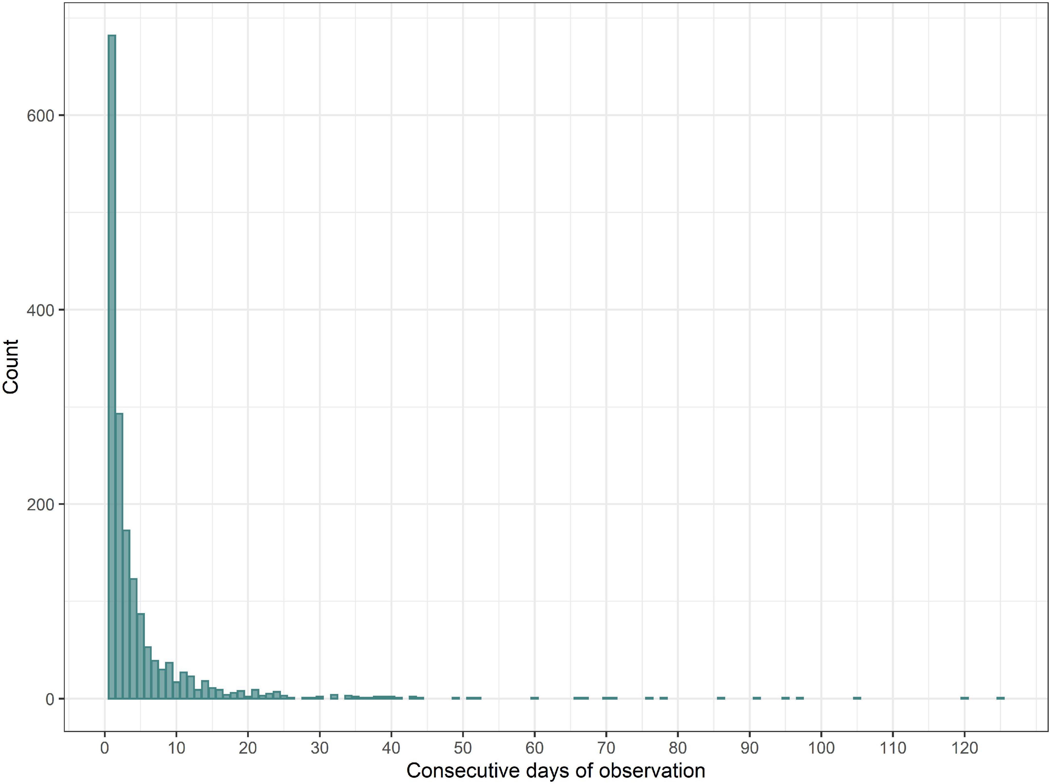
Figure 4. Frequency distribution for length of runs of consecutive observation days. One outlier (length of the run = 276 days) has been excluded.

Analysis of species occurrence records during runs of consecutive observation days (at the same site), using the site-date dataset (Subset B), showed that non-independence was evident at time-lags of (at least) up to 8–10 days. For bottlenose dolphin, correlations above r = 0.3 are seen for lags of 1–10 days while, for other species, correlations were above r = 0.2 for lags up to 8 or 9 days. There were insufficient data for longer runs to adequately test for autocorrelation at longer time-lags. The analysis does not provide a measure of autocorrelation in sighting rate results per se (it is based on combined data for all site-dates and not on analysis of individual runs of which, as noted above, there are many, mostly very short) but it indicates that species occurrences at a site on consecutive days are not independent.

Utility of Consecutive Watches

The analysis of the sighting rates over consecutive watches, again performed with Subset A, showed that there were no consistent trends in the mean sighting rate, or its variance, over the watches carried out during a day. The analysis of the cumulative sighting rates reveals that the estimates become more similar and their variance decreases (i.e., precision increases) as more watches are carried out in a day. Nonetheless, the additional benefits from each successive watch also decrease: while there is a noticeable gain in the consistency and precision of sighting rate estimates from 1 to 5 watches, the benefit from performing the 10th watch after performing nine watches is much reduced. Note that while these results suggest there is value in carrying out 5 or more successive watches, the absolute values of variance obtained should be treated with caution since there is autocorrelation in the data.

Does Observation “Success” Influence Observer Behavior?

No significant differences were observed between mean sighting rates (of all cetacean species together) for those watches which were immediately followed (i.e., after 1 h) by another watch (mean = 0.17; 95% CI 0.14–0.19; N = 842) and those watches which were followed by a gap in data collection (mean = 0.18; 95% CI 0.18–0.24; N = 269). Thus, there is no evidence that the decision of observers to stay was conditioned by the sighting(s) of animals during the first watch. It may be noted that first watches followed by a consecutive watch were three times more numerous (N = 842) than those not followed by a consecutive watch (N = 269).

In addition, no significant correlation was observed between the sighting rate in the first watch and the number of following consecutive watches (r = −0.03; p = 0.88), nor between the number of animals seen in the first watch and the number of consecutive watches (r = −0.02; p = 0.27). Hence, in general, the decision of observers to stay at the observation site was apparently not influenced by the number of animals observed in the first watch.

Ability to Detect Changes in Sighting Rates

The power to detect downward trends in sighting rate (a proxy for local abundance) over a series of years is a function of the initial sighting rate for each species, the underlying rate of decline and the number of watches per year (among other factors). Our simulations considered these three variables and used two possible metrics: the likelihood of obtaining a statistically significant (p < 0.05) trend and the likelihood of the rate of decline detected being at least as steep as the underlying rate of decline (within a limit of tolerance).

In this study, the mean sighting rate for most species was quite low, ranging between 0.115 sightings per watch (SD = 0.042) and 0.004 (SD = 0.008) for bottlenose dolphin and common dolphin, respectively (Table 6).

TABLE 6

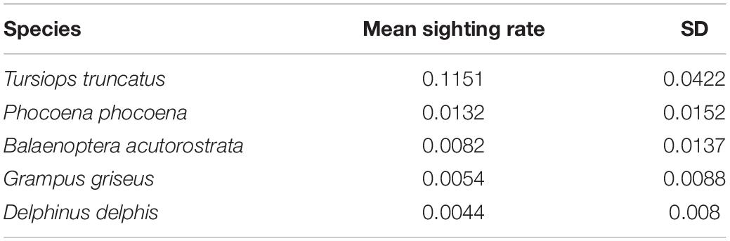
Table 6. Mean sighting rate and standard deviation for each of the studied species.

The lower the initial sighting rate (prior to a decline), the higher the number of watches needed to detect a statistically significant decline over 6-year period on at least 95% of occasions (Figure 5A). Thus, to be 95% sure of detecting a negative trend when simulating a 60% decline, it would be necessary to perform 430 watches per year for bottlenose dolphin (sighting rate = 0.11, SD = 0.042) but more than 4000 watches for harbor porpoise (sighting rate = 0.013, SD = 0.015), implying that such decline could not be detected. If we set the required certainty at 80% (but retaining the 95% statistical significance level), 260 watches per year and 2870 watches per year would be necessary, respectively. To detect a smaller negative trend, e.g., 30% with 95% of certainty (at a 95% significance level) for bottlenose dolphin (sighting rate = 0.11), it would be necessary to perform 1990 watches per year or 1230 if we set the required certainty at 80%. The results of the simulations for other rates of decline can be found in Supplementary Figure 4.

FIGURE 5

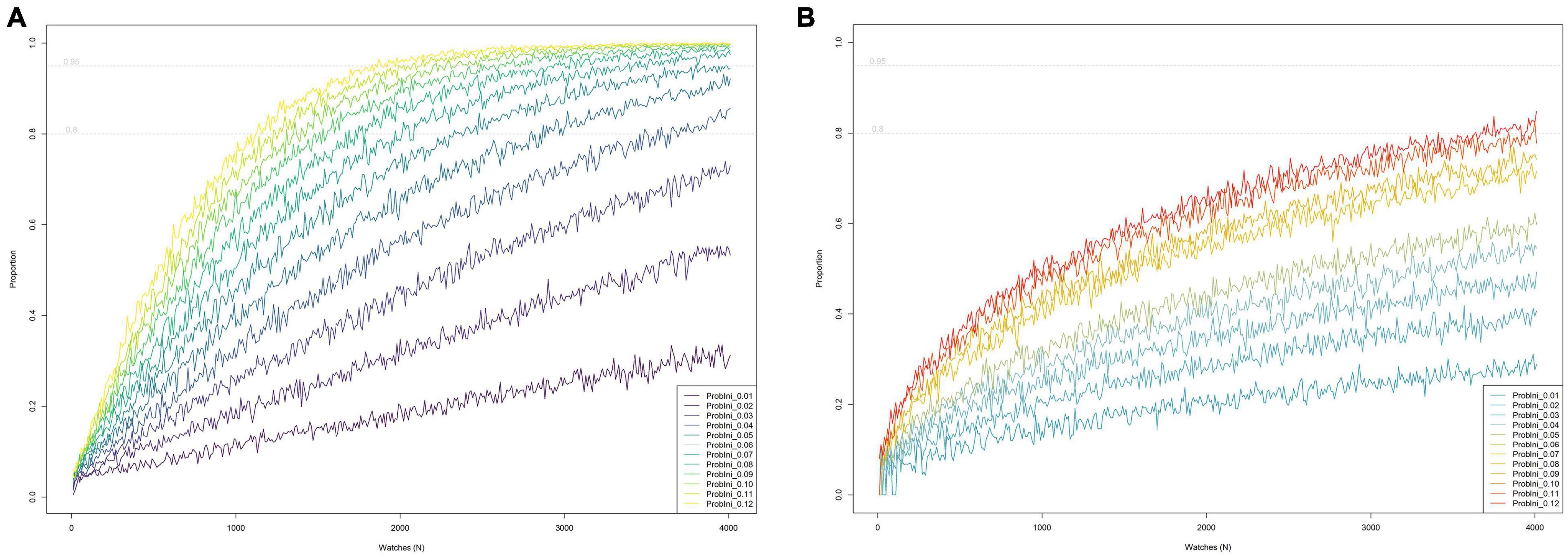
Figure 5. The relationship between the annual number of watches (based on the notional approach of all these watches occurring at a single site with a known underlying initial sighting rate) and the proportion of simulations during which “trend detection criteria” were met, given an overall decline in sighting rate of 30% over 6 years, for a range of values for initial sighting rates (i.e., a range of initial values for relative abundance). Dotted horizontal gray lines indicate where 80 and 95% detection success was achieved. (A) Using the criterion that a statistically significant decline is detected (regardless of the estimated regression slope). (B) Using the criterion that the estimated regression slope is equivalent to a decline equal to or greater than the true underlying rate of decline over 6 years (in this example 30%), applying a tolerance limit of 20%. Thus the estimated slope must be equivalent to a decline of at least 24% over 6 years (since 20% of 30% is 6% and 30–6% = 24%).

If we focus on the rate of decline, the number of watches required (to achieve 95% certainty of recording a rate of decline at least as great as the true underlying rate of decline, given a margin of tolerance) increased considerably compared to that suggested by the previous approach (Figure 5B). Thus, to detect a 30% decline (with a tolerance limit of 20% of the true rate, i.e., to detect a decline of at least 24%) on 80% of occasions, it would be necessary to perform 3840 watches per year for bottlenose dolphin (sighting rate = 0.11) and more than 4000 watches per year for harbor porpoise (sighting rate = 0.013), meaning that such percentage of decline will not be detected. Obviously, setting more stringent criteria (in terms of tolerance limits or the probability that the regression slope is at least as steep as that defined by the tolerance limit), will require a higher number of watches per year, especially for those species with lower sighting rates. The results of the simulations using different values can be found in Supplementary Figure 5.

It should be noted that carrying out a certain number of watches obviously does not guarantee that a certain rate of population decline will be detected by a given statistical test–but the likelihood of a statistical test failing to detect a real trend (i.e., a type II error) evidently decreases as the number of watches increases. A second caveat is that the validity of the statistical tests depends on results from each watch being independent of results from other watches, so (for each year) watches would ideally need to be spread across multiple sites and over the whole year–and since this might in turn lead to a change in the underlying sighting rate, the number of watches needed would have to be adjusted accordingly.

Patterns and Trends in Cetacean Sightings

For each cetacean species, the explanatory variables that had significant effects on each response variable are presented in Table 7, as well as the model diagnostics. The results of the models for each response variable for a given cetacean species are expected to show some differences since the factors influencing or determining the number of animals in a group (group size) might not be the same as those influencing its occurrence or the number of groups sighted. GAM plots are available in Supplementary Figures 8–30.

TABLE 7

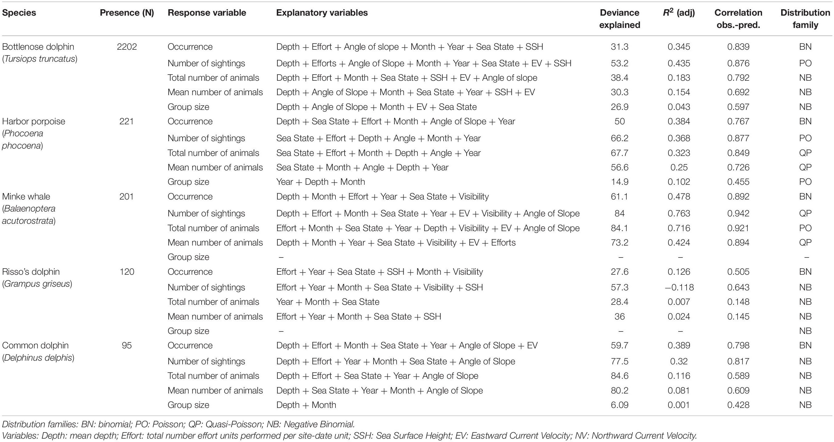
Table 7. Models results for each species: number of presences, response variables, explanatory variables selected by the models (in descending order of importance according to deviance explained), total deviance explained, R² adjusted, correlation between the observed and the predicted values and distribution family used.

Bottlenose Dolphin

Models for bottlenose dolphin show a strong influence of the mean sea depth in the area around the observation sites (14.77% of the total deviance explained (DE) for occurrence, as determined by comparing models with and without this variable included; 30.86% DE for the number of sightings in a day and 19.05% DE for mean number of animals sighted), with maximum values being seen over mean depths of around 30 m. Group size is also influenced by mean depth but with a lower deviance explained (3.10%).

Other significant explanatory variables were: (1) mean angle of slope of the seabed (5.2% DE for occurrence, 13.63% DE for the number of sightings in a day and 6.99% DE for mean number of animals sighted); (2) month (3.57% DE for occurrence, 5.51% DE for number of sightings per day and 2.36% for mean number of animals sighted), presenting a peak between May and July; and (3) the number of watches in each site-date unit, which mainly influenced occurrence (5.78% DE) and mean group size (1.47% DE).

The observation sites with the highest probability of occurrence of bottlenose dolphin are: Torry Battery (Aberdeen) (0.548, SD = 0.189), Chanonry Point (0.456, SD = 0.211), Spey Bay (0.433, SD = 0.262), North Kessock (0.175, SD = 0.165), Macduff (0.125, SD = 0.639), and Cullen (0.079, SD = 0.053). Bottlenose dolphin occurrence presented a decreasing year-on-year trend (a decline of 0.007 in probability of occurrence per year) whilst the mean number of animals sighted presented an increase (an increase of 0.059 in the mean number of animals sighted).

Harbor Porpoise

Harbor porpoise models show that mean depth was the variable with the greatest influence on occurrence (22.99% DE) and on the number of sightings in a day (22.17% DE), both of which increased as the depth increases. This was followed by sea state, the number of watches performed in a day, and the month, with a slight decrease in June–July. By contrast, the total and the mean number of animals sighted were mainly influenced by sea state (31.42% DE and 31.26% DE, respectively), with a lower probability of detection at higher sea states, followed by the month, with a higher probability of occurrence between June and September. Mean group size and the mean number of animals per sighting, were mainly influenced by the year (6.9% DE), with an increase being seen from 2015 onward.

The observation site with the highest probability of occurrence of harbor porpoise is Tiumpan Head (Isle of Lewis) (0.156, SD = 0.123), with much lower probabilities at other observation sites–ranging from 0.009 in Macduff to 0.0007 in North Kessock. Harbor porpoise occurrence and mean number of animals sighted present a weakly increasing trend since 2013 (an increase of 0.006 in the probability of occurrence per year; an increase of 0.004 in the mean number of animals sighted per year).

Minke Whale

Models for minke whale also show a strong influence of mean depth on most of the response variables (total number of sightings 53.49% DE; mean number of animals 21.16% DE; mean group size 49.62% DE), the effect of increasing depth being positive at depths greater than 60 m. Occurrence was mainly influenced by the number of watches (42.97% DE). Other significant explanatory variables are: (1) month (9.51% DE for occurrence; 5.68% DE for mean number of animals sighted; 7.89% DE for occurrence and 9.96% for mean group size), presenting a peak between May and July, and (2) sea state, which generally had a negative effect on the number of sightings and mean number of animals sighted (6.29 and 2.53%).

The observation site with the highest probability of occurrence of minke whale is Tiumpan Head (0.169, SD = 0.193). Over the study period, this species presented a year-on-year increasing trend in occurrence and mean number of animals sighted yearly (occurrence: rate = 0.009, i.e., an increase of 0.009 in the probability of occurrence per year; mean number of animals sighted: rate = 0.006, i.e., an increase of 0.006 in the mean number of animals sighted).

Risso’s Dolphin

The fits obtained for Risso’s dolphin models were poor compared with those for the above-mentioned species, but the models show that occurrence, number of sightings and mean number of animals sighted were mainly influenced by the number of watches (13.19% DE, 19.7% DE, and 8.33% DE, respectively). Year was a significant explanatory variable for all the response variables (% DE ranging from 4.39% for mean group size to 15.99% for the number of sightings), with an increase being seen from 2015 onward.

The observation sites with the highest probabilities of Risso’s dolphin occurrence were Tiumpan Head (0.019, SD = 0.003) and Spey Bay (0.008, SD = 0.012). Probability of occurrence was lower (<0.007) at Torry Battery, North Kessock, and Macduff. Occurrence and mean number of animals sighted yearly both increased over the course of the study period (an increase of 0.008 in the probability of occurrence per year; an increase of 0.013 in the mean number of animals sighted).

Common Dolphin

Common dolphin models also performed poorly, nonetheless showing that the main explanatory variable influencing all the response variables was the mean depth (51.55% DE for number of sightings, 21.52% for mean number of animals, 14.82% for occurrence, 40.77% for mean group size), with values of all response variables being higher as the depth increases.

The observation site with the highest probability of occurrence of common dolphin is Tiumpan Head (0.078, SD = 0.069). Occurrence and mean number of animals sighted showed an increasing trend over the course of the study period (an increase of 0.004 in the probability of occurrence per year; an increase of 0.012 in the mean number of animals sighted).

Group Size Variation

Mean group size (number of animals sighted divided by the number of sightings, per site-date unit) shows high seasonal variation in bottlenose dolphin, ranging from groups of two individuals on average in winter months to groups of up to eight individuals in June–July. Harbor porpoise and minke whale also show some seasonal variation in mean group size, the former showing an increase in the group size in July and October and the latter showing an increase in June. Risso’s dolphin and common dolphin showed little seasonal variation in group size.

Mixed Models

Fitted GAMMs for sighting rate and for occurrence of bottlenose dolphin, using an AR(1) structure, did not markedly change the goodness of fit compared to GAMs (GAM sighting rate–R² = 0.309, dispersion (disp) = 0.568; GAMM sighting rate–R² = 0.272, disp = 0.710; GAM occurrence–R² = 0.408, disp = 1.013; GAMM occurrence–R² = 0.403; disp = 1.075). Model diagnostics were satisfactory for both models, e.g., no apparent relationships of residuals with explanatory variables and the same explanatory variables in both modeling approaches were significant. For the remaining species, mixed models did not converge.

Discussion

The WDC Shorewatch program has generated a substantial amount of observation effort distributed along the Scottish coast, especially since 2012. During the time period considered here (2015–2018), this citizen science project has generated almost 9000 h of observation effort and a very large number of sightings of the coastal cetacean species of Scotland–species which are protected under the EU Habitats Directive (Council Directive 92/43/EEC,), thus offering a potentially valuable monitoring tool. Shorewatch contributed to the proposal and subsequent designation of a Marine Protected Area (MPA), namely the North-East Lewis Nature Conservation MPA, particularly by providing data on winter sightings. Shorewatch data can be used to demonstrate inter-annual and inter-site variation in bottlenose dolphin sightings in a SAC (Embling et al., 2015) as well as more widely for harbor porpoise, minke whale and Risso’s dolphin (Weir et al., 2019). As demonstrated in this study, they can be used to detect patterns, trends and changes in sighting rates of regularly sighted species.

The observation effort carried out under this program is to a considerable extent concentrated in a few observation sites as well as occurring mainly during times of the year and times of the day when observation conditions are more favorable. It would thus be desirable to achieve a more evenly distributed effort across the active observation sites and to increase it toward both ends of the year and indeed toward dawn and dusk. Apart from providing a more rounded picture of use of the Scottish coast by cetaceans, a wider distribution of effort might also have the beneficial consequence of reducing the amount of autocorrelation in the dataset or at least allowing it to be taken into account, and of increasing the data’s utility for providing robust indicators of status and changes in status of cetaceans. While changes in the observation sites used were almost inevitable as the utility of initially selected sites was evaluated, it will be important to maintain at least a core set of sites to help ensure the consistency of the data collected.

While the WDC Shorewatch protocol is well-established and is designed to ensure consistency of data collection (e.g., the program involves the training of citizen volunteers), some aspects of the protocol are difficult to evaluate and some error and/or bias could arise due to observer behavior and motivation. Between-observer variability may occur in detecting cetaceans, identifying species, counting cetacean numbers and describing weather conditions. Although observers are provided with training in order to reduce such variability, it would be worthwhile to analyze subsets of data from known observers to test this.

To the extent that we were able to evaluate this, we found no evidence of observer-related bias in the data. For example, we found no evidence that the sighting of animals (or the number sighted) during a watch influences observers’ decision to stay at the observation site. It should be noted that the decisions of the volunteers can be influenced by many factors. The Shorewatch program involves many different people and covers a diverse study area. In addition, the number of volunteers involved in carrying out the watches on a particular day at a particular site is variable, and individuals may come and go during a sequence of watches. Further analysis could look at results for specific (named) observers.

Temporal autocorrelation is evident in the sightings data. There is evidence of autocorrelation both between successive watches and between successive days. This autocorrelation is a consequence of both the behavior of the species observed and the methodology employed (e.g., carrying out consecutive watches at a site). Thus, coastal bottlenose dolphins tend to use the same areas, day after day, year-round (Wilson et al., 1997, 2004; Stockin et al., 2006; Culloch and Robinson, 2008; Dinis et al., 2016). Hence, consistent occurrence or lack of occurrence at a site is precisely what might be expected of most and least preferred sites, respectively. Of course, understanding the reason for autocorrelation does not mean that it is not an issue for statistical analysis.

The consistency and apparent precision of estimated sighting rate increases when using data from several consecutive watches, while autocorrelation will be reduced if we join data from consecutive watches. Given that, it could be argued that the best approach is to estimate a cumulative (or average) sighting rate across all watches in a day, as done for the present analysis. Indeed, doing this for multiple days could provide more suitable data for revealing long-term trends in local occupancy or abundance.

As the current 1 h lag between watches does not seem to remove temporal autocorrelation, rather than 60 min of observation time comprised of six 10-min watches spread over 10 h, could equally valuable information be obtained from, for example, 60 consecutive minutes of observation or three 20-min watches, or other possible combinations? An obvious advantage of the maintaining the current approach is that data are more likely to be spread across different times of day and at different stages of the tidal cycle. However, longer watches could have benefits such as reducing the probability of missing cetaceans that are present or increasing the motivation of some volunteers. Fewer, longer watches could be more appropriate if the objective is to study patterns of occurrence over short time-scales, e.g., in relation to tidal cycles, or to build a more detailed picture of the activity budgets of the animals. It could also provide a more enjoyable experience for those volunteers who are able to participate less frequently but are able to spend more time making observations on those days when they are available. The desirability of minimizing within-day temporal autocorrelation should also be borne in mind. If there is more than one watch at a site per day, autocorrelation will not be avoided but post hoc data processing (e.g., joining data from consecutive watches) can reduce or even eliminate it.

Continuing with 10-min watches would arguably maintain a reasonable balance between achieving monitoring objectives and providing a satisfactory volunteer experience of observation (as well as meeting the needs of volunteers who do not have increased time to offer). Furthermore, short watches avoid observer fatigue and help the volunteers to keep focused during the whole watch, minimizing the likelihood of missing a sighting. Thus, the results of the watches should give a more accurate picture of the situation in the field, in term of number and species present, and help to ensure a uniform detection rate during each watch.

Retaining the 10-min watch also has the big advantage of preserving the integrity of the data series. It might be useful however, to suggest optional additional tasks for observers to carry out during some of the 50-min “resting” period between watches, e.g., collecting behavioral or activity budget data or observing interspecies interactions.

The Shorewatch program is being rolled out in the northern islands of Scotland and the likely lower rate of cetacean sightings has led to questions about whether the protocol could be modified to account for this. In order to maintain comparability with historical data, one compromise option would be to propose (say) 20-min watches, with hourly intervals between the starting times of each watch. This would help adjust to the different conditions, while data equivalent to the existing series could be extracted by using only data from the first 10 min of each watch.

Ability to Detect Changes in Sighting Rate

The simulations performed were carried out with the intention of setting a minimum level of effort at which trends in local abundance could realistically be detected. Therefore, they could help to identify how many watches are needed to detect a decline (or a certain rate of decline) over a 6-year period (as required for use in assessment of GES under the MSFD). The answer is obviously dependent on the typical sighting rate for the species and the rate of decline that needs to be detected.

Inevitably, the conclusion depends on the criterion selected and there is no approach which could provide 100% assurance that a statistically significant decline (or a particular rate of decline) would be detected. In this case, we considered two options. The first involved detecting a statistically significant (p < 0.05) trend over 6 years, 95% (or 80%) of the time. We used linear regression rather than correlation, since the former allows an overall rate of decline (or increase) to be estimated, even if the trend appears to be non-linear. This method, used to quantify the rate of decline, is likely to perform adequately for low rates of decline. For higher rates of decline, it will be more evident that abundance follows an exponential curve: as the population falls, the annual change in population size, which is a percentage, also falls. Fitting a linear regression will then be an increasingly inaccurate way of depicting the change. Our second approach focused on the need to determine whether a decline of at least X% had taken place over 6 years. We approached this by setting a tolerance limit (L), so that a decline of at least X-L% had to be detected 95% (or 80%) of the time. These latter simulations suggested that higher numbers of watches would be needed, as this is a more stringent test.

In theory, a statistically more robust estimate of any downward trend in abundance could be derived from the habitat models, in which year is an explanatory variable and effects of other explanatory variables are also taken into account. However, caution is also needed: while it clearly makes sense to account for changes in detectability, if, for example, the year-to-year trend in sighting rate is well explained by changes in temperature (and year thus drops out of the model), evidently it does not mean that no change in sighting rate took place.

For this analysis, sighting rate (calculated as the mean number of sightings per watch per site-date unit) was used since it is less likely to be affected by variation in the detection skills between observers than metrics which rely on the count of the animals sighted (Thompson et al., 2000). It was assumed that each watch is a valid and independent estimate of the underlying sighting rate. If the requisite number of watches can be spread not only over the whole year but also across all sites, this would help to ensure independence of the data as well as providing a more robust view of any trends. By basing the simulation on results from a single site, we have oversimplified the situation. Sighting rates differ between sites which will affect the overall average sighting rate for each species and, consequently, the estimate of the required number of watches. It should also be borne in mind that if the distribution of observers across sites changes from year to year, this could also generate changes in average sighting rates. This needs to be controlled, perhaps at the time of data collection or alternatively via post hoc standardization of the data.

The 6-year time window used for the calculations, to detect trends in cetacean abundance, was based on the reporting cycles of the MSFD and the Habitats Directive. Such simulations results could act as a guideline to set effort objectives for different monitoring purposes, depending on the amount or rate of decline which needs to be detected, and on the sighting characteristics of the species in the study area. In future, synchronization of the analysis of the sightings data with Habitats Directive or MSFD reporting periods could make the data collected by the WDC Shorewatch program more useful to conservation managers. To this end, we recommend that subsequent analysis takes place in synchrony with these 6-yearly reporting cycles.

Patterns and Trends in Cetacean Sightings

The total number of sightings varied between the five coastal cetacean species studied (i.e., bottlenose dolphin, harbor porpoise, minke whale, Risso’s dolphin, and common dolphin), affecting to the ability of the models to detect relationships with the explanatory variables. Thus, for those species with a greater number of sightings, such as bottlenose dolphin and harbor porpoise, we obtained models that are more reliable (in terms of descriptive and, potentially, predictive power). We selected a subset of the data containing those sites at which effort is more regularly distributed over time–within and between years–and with the longest possible time series. Almost all of the sites thus selected for the study of trends [i.e., Chanonry Point, North Kessock, Spey Bay, Cullen, Macduff, and Torry Battery (Aberdeen)], are located in the east coast of Scotland, with the exception being Tiumpan Head. This undoubtedly reflects the location of WDC supporting staff during the early years of the program but it also highlights the need to improve the observer coverage at sites on the west and north coasts. The Scottish coast is topographically diverse and each observation site has distinctive characteristics (platform height, field of view or the mean depth of the surrounding water). We did not include all these characteristics in the models, partly because they are likely to be correlated with each other and partly because we would need to include more sites to start to tease apart the relative contributions of the different variables. Despite these limitations, the analysis completed demonstrates the utility of the data collected by the Shorewatch program.

The data collected offer several different metrics for use as response variables, such as occurrence, number of sightings per site-date unit, total number of animals sighted per unit or group size, the analysis of which provides complementary information.

The different cetacean species considered presented different spatial and seasonal distribution patterns in the seven studied locations. Usually, in those places or seasons where bottlenose dolphins are present, other species such as harbor porpoise, minke whale and common dolphin are either absent or show a different seasonal distribution. This could be due to avoidance behavior or temporal habitat partitioning between species. For example, harbor porpoise might be expected to avoid those time/area combinations associated with bottlenose dolphin presence, as a way to avoid fatal attacks by bottlenose dolphins (Thompson et al., 2004).

Bottlenose dolphins are mainly present in the observation sites located on the East coast [Chanonry Point, North Kessock, Spey Bay, Cullen, Macduff, and Torry Battery (Aberdeen)], being uncommon at Tiumpan Head (Isle of Lewis, Outer Hebrides), as also stated by Weir et al. (2001). North Kessock and Chanonry Point are both located in the Moray Firth, a core part of the range of the resident population and where year-round bottlenose dolphin presence has been previously demonstrated (Wilson et al., 1997). The seasonal differences observed in the group size of bottlenose dolphin are consistent with changes observed by Wilson et al. (1997), with the largest group sizes seen from May to September and the lowest from October to April, probably linked to seasonal changes in use of the area by the dolphins (e.g., linked to the reproductive cycle).

The seasonality observed in minke whale occurrence, seen most often at Tiumpan Head, is consistent with peak abundance between June and August described by Weir et al. (2001) for the east coast of Lewis. Previous studies describe similar seasonal patterns of minke whale occurrence on the East coast of Scotland, in the outer part of Moray Firth (Tetley et al., 2008; Robinson et al., 2009), with the distribution of sightings varying according to prey availability in the area (Robinson and Tetley, 2007). The Southern Trench Nature Conservation MPA has recently been designated for minke whale. Although, in this study, five observation sites were situated in the Moray Firth (Chanonry Point, North Kessock, Spey Bay, Cullen, and Macduff), the results of the models suggest a low presence of minke whales in this area. It is likely that a more offshore distribution of the minke whale and their prey could make the detection of the species difficult from shore-based observation points, whereas minke whale may be more easily detected from boat surveys (as in Robinson and Tetley, 2007, Robinson et al., 2009).

Model predictions of both occurrence and number of sightings showed upward long-term trends over the period 2012–2018, for four of the five studied species, with the exception being bottlenose dolphin. It will be necessary to investigate in more detail whether this could be an artifact of the changes in the distribution of the observations in space and time or if it is a genuine increase of occupancy and/or abundance of these species in Scottish coastal waters. Evidently year-to-year and seasonal changes at the studied sites may reflect changes in the distribution of the species rather than changes in its abundance. It is also the case that the explanations for such changes may involve factors not considered in the present study, such as changes in prey availability, anthropogenic disturbance, or inter-specific competition between cetacean species (Ross and Wilson, 1996; Thompson et al., 2004). Continued ocean warming could result in changes in cetacean communities in Scotland, with increased presence of species typically found in warmer waters, such as striped dolphin (Stenella coeruleoalba) (Lambert et al., 2014), Risso’s dolphin and common dolphin (MacLeod et al., 2005; Stockin et al., 2006; Robinson et al., 2010) coupled with reduced occurrence of species more typical of cooler waters, such as minke whale and white-beaked dolphin (Lagenorhynchus albirostris) (MacLeod et al., 2005, 2008). By contrast, bottlenose dolphin presented a downward long-term trend in mean local occurrence and mean number of sightings in the present study, as also seen by Culloch and Robinson (2008) during 2001–2004 in the Moray Firth. Previous studies have suggested that animals from the Moray Firth bottlenose population have increasingly been seen off Aberdeenshire and further south toward the Firth of Forth (e.g., Stockin et al., 2006), but also that the use of the latter areas may fluctuate seasonally and over longer time-scales. Thus, mark-recapture studies suggest that the part of the population in the Moray Firth was stable or increasing between 1990 and 2010 and between 2014 and 2016 (Cheney et al., 2014, 2018; ICES, 2016) and that the part of the population present in St. Andrews Bay and the Tay Estuary increased between 2009 and 2015 during the summer season (Arso Civil et al., 2019).

The models showed that the explanatory variable with the largest influence on occurrence and the number of sightings was the mean depth of water in the vicinity of the study area, except in the case of Risso’s dolphin. Sea depth close to the coast was also an important factor in determining land-based sighting rates for coastal cetaceans on the Northwest Spanish coast (Pierce et al., 2010), presumably in part because it determines the extent to which deeper water species approach to the coast. This needs further investigation in this dataset but coastal water depth could potentially be included as a factor when considering potential new Shorewatch observation sites. Since it reflects the local geomorphology, this variable may also likely to be related to the height of the observation site (Supplementary Table 1).

The WDC Shorewatch program, with its standardized data collection, offers a valuable source of information about coastal cetaceans in Scotland which has already contributed data for the designation of NE Lewis Nature Conservation MPA (Scottish Ministerial Order, 2020) and has influenced the timing of works for development activities in coastal waters (so as to minimize disturbance to bottlenose dolphins). It provides data that can be used to detect trends in local occurrence and relative abundance and to study the temporal and spatial distribution of five cetacean species. In addition, because it also collects data on species other than those studied in this paper, Shorewatch can support a range of other studies on coastal wildlife in Scotland. Furthermore, this ongoing citizen science program continues to collect data, building upon the data set used in the current analysis. As a long-term monitoring initiative, it aims to inform management bodies about the relative state of coastal cetacean sightings over time, and thus to meaningfully contribute to cetacean conservation.

Data Availability Statement

The raw data supporting the conclusions of this article will be made available by the authors, on request, subject to a data sharing agreement.

Ethics Statement

Ethical review and approval was not required for the animal study because the study is based on coastal observation of cetaceans which were performed without approaching or disturbing to the animals.

Author Contributions

All authors contributed to defining the aims of the present analysis and designing the detailed content. AW maintained and provided the data. GP and PG-M designed and carried out the statistical analysis and wrote the manuscript with contributions from AW and SD.

Funding

This work was funded by Whale and Dolphin Conservation (WDC) and NatureScot (formerly Scottish Natural Heritage).

Conflict of Interest

The authors declare that the research was conducted in the absence of any commercial or financial relationships that could be construed as a potential conflict of interest.

Publisher’s Note

All claims expressed in this article are solely those of the authors and do not necessarily represent those of their affiliated organizations, or those of the publisher, the editors and the reviewers. Any product that may be evaluated in this article, or claim that may be made by its manufacturer, is not guaranteed or endorsed by the publisher.

Acknowledgments

Thanks are due to all the volunteers of the Shorewatch program, who spent many hours in the field, for their dedication and outstanding commitment to data collection and cetacean conservation. Especial thanks are due to Katie Dyke for her leadership and support of Shorewatch volunteers and field work. The authors also gratefully acknowledge the editorial input of Karen Hall and Morven Carruthers to the report on which this manuscript is based and the very useful input from referees. Furthermore, the authors acknowledge support by the CSIC Open Access Publication Support Initiative through its Unit of Information Resources for Research (URICI).

Supplementary Material

The Supplementary Material for this article can be found online at: https://www.frontiersin.org/articles/10.3389/fmars.2021.642386/full#supplementary-material

References

Anderwald, P., Evans, P. G., Dyer, R., Dale, A., Wright, P. J., and Hoelzel, A. R. (2012). Spatial scale and environmental determinants in minke whale habitat use and foraging. Mar. Ecol. Prog. Ser. 450, 259–274. doi: 10.3354/meps09573

CrossRef Full Text | Google Scholar

Arso Civil, M., Quick, N. J., Cheney, B., Pirotta, E., Thompson, P. M., and Hammond, P. S. (2019). Changing distribution of the east coast of Scotland bottlenose dolphin population and the challenges of area-based management. Aquat. Conserv. Mar. Freshw. Ecosyst. 29, 178–196. doi: 10.1002/aqc.3102

CrossRef Full Text | Google Scholar

Avila, I. C., Kaschner, K., and Dormann, C. F. (2018). Current global risks to marine mammals: taking stock of the threats. Biol. Conserv. 221, 44–58. doi: 10.1016/j.biocon.2018.02.021

CrossRef Full Text | Google Scholar

Bailey, H., Corkrey, R., Cheney, B., and Thompson, P. M. (2013). Analyzing temporally correlated dolphin sightings data using generalized estimating equations. Mar. Mamm. Sci. 29, 123–141. doi: 10.1111/j.1748-7692.2011.00552.x

CrossRef Full Text | Google Scholar

Bailey, H., and Thompson, P. (2010). Effect of oceanographic features on fine-scale foraging movements of bottlenose dolphins. Mar. Ecol. Prog. Ser. 418, 223–233. doi: 10.3354/meps08789

CrossRef Full Text | Google Scholar

Baird, R. W. (2009). “Risso’s dolphin: Grampus griseus,” in Encyclopedia of Marine Mammals, eds H. Thewissen, B. Würsig, and W. F. Perrin (Cambridge, MA: Academic Press), 975–976. doi: 10.1016/B978-0-12-373553-9.00222-4

CrossRef Full Text | Google Scholar

Baulch, S., and Perry, C. (2014). Evaluating the impacts of marine debris on cetaceans. Mar. Pollut. Bull. 80, 210–221. doi: 10.1016/j.marpolbul.2013.12.050

PubMed Abstract | CrossRef Full Text | Google Scholar

Becker, J. J., Sandwell, D. T., Smith, W. H. F., Braud, J., Binder, B., Depner, J., et al. (2009). Global bathymetry and elevation data at 30 Arc seconds resolution: SRTM30_PLUS. Mar. Geodesy 32, 355–371. doi: 10.1080/01490410903297766

CrossRef Full Text | Google Scholar

Bouchet, P. J., Thiele, D., Marley, S. A., Waples, K., Weisenberger, F., Rangers, B., et al. (2021). Regional assessment of the conservation status of snubfin dolphins (Orcaella heinsohni) in the Kimberley region, Western Australia. Front. Mar. Sci. 7:1222. doi: 10.3389/fmars.2020.614852

CrossRef Full Text | Google Scholar

Cheney, B., Corkrey, R., Durban, J. W., Grellier, K., Hammond, P. S., Islas-Villanueva, V., et al. (2014). Long-term trends in the use of a protected area by small cetaceans in relation to changes in population status. Glob. Ecol. Conserv. 2, 118–128. doi: 10.1016/j.gecco.2014.08.010

CrossRef Full Text | Google Scholar

Cheney, B., Graham, I. M., Barton, T. R., Hammond, P. S., and Thompson, P. M. (2018). Site Condition Monitoring of bottlenose dolphins within the Moray Firth Special Area of Conservation: 2014-2016. Scottish Natural Heritage Research Report 1021. Inverness: NatureScot Government agency.

Google Scholar

Cheney, B., Thompson, P. M., and Cordes, L. S. (2019). Increasing trends in fecundity and calf survival of bottlenose dolphins in a marine protected area. Sci. Rep. 9, 1–9. doi: 10.1038/s41598-018-38278-9

PubMed Abstract | CrossRef Full Text | Google Scholar

Cheney, B., Thompson, P. M., Ingram, S. N., Hammond, P. S., Stevick, P. T., Durban, J. W., et al. (2013). Integrating multiple data sources to assess the distribution and abundance of bottlenose dolphins Tursiops truncatus in Scottish waters. Mamm. Rev. 43, 71–88. doi: 10.1111/j.1365-2907.2011.00208.x

CrossRef Full Text | Google Scholar

Council Directive 92/43/EEC of 21 May 1992 on the conservation of natural habitats and of wild fauna and flora. Official Journal L 206, 0007-0050. Available from: http://eur-lex.europa.eu/.

Google Scholar

Cox, S., Embling, C. B., Hosegood, P. J., Votier, S. C., and Ingram, S. N. (2018). Oceanographic drivers of marine mammal and seabird habitat-use across shelf-seas: a guide to key features and recommendations for future research and conservation management. Estuar. Coast. Shelf Sci. 212, 294–310. doi: 10.1016/j.ecss.2018.06.022

CrossRef Full Text | Google Scholar

Culloch, R. M., and Robinson, K. P. (2008). Bottlenose dolphins using coastal regions adjacent to a Special Area of Conservation in north-east Scotland. J. Mar. Biol. Assoc. U.K. 88:1237. doi: 10.1017/S0025315408000210

CrossRef Full Text | Google Scholar

de Boer, M. N., Simmonds, M. P., Reijnders, P. J., and Aarts, G. (2014). The influence of topographic and dynamic cyclic variables on the distribution of small cetaceans in a shallow coastal system. PLoS One 9:e86331. doi: 10.1371/journal.pone.0086331

PubMed Abstract | CrossRef Full Text | Google Scholar

Dinis, A., Alves, F., Nicolau, C., Ribeiro, C., Kaufmann, M., Cañadas, A., et al. (2016). Bottlenose dolphin Tursiops truncatus group dynamics, site fidelity, residency and movement patterns in the Madeira Archipelago (North-East Atlantic). Afr. J. Mar. Sci. 38, 151–160. doi: 10.2989/1814232X.2016.1167780

PubMed Abstract | CrossRef Full Text | Google Scholar

Directive 2008/56/EC of the European Parliament and of the Council of 17 June 2008 Establishing a Framework for Community Action in the Field of Marine Environmental Policy (Marine Strategy Framework Directive). OJ L 164/19. Available online at: http://eur-lex.europa.eu/.

Google Scholar

Dolman, S. J., Hodgins, N. K., MacLeod, C. D., Pierce, G. J., and Weir, C. R. (2014). Harbour porpoises (Phocoena phocoena) and minke whales (Balaenoptera acutorostrata) observed during land-based surveys in The Minch, north-west Scotland. J. Mar. Biol. Assoc. U.K. 94, 185–194. doi: 10.1017/s0025315413000507

CrossRef Full Text | Google Scholar

Dormann, C. F., Elith, J., Bacher, S., Buchmann, C., Carl, G., Carré, G., et al. (2013). Collinearity: a review of methods to deal with it and a simulation study evaluating their performance. Ecography 36, 27–46. doi: 10.1111/j.1600-0587.2012.07348.x

CrossRef Full Text | Google Scholar

Embling, C. B., Walters, A. E. M., and Dolman, S. J. (2015). How much effort is enough? The power of citizen science to monitor trends in coastal cetacean species. Glob. Ecol. Conserv. 3, 867–877. doi: 10.1016/j.gecco.2015.04.003

CrossRef Full Text | Google Scholar

Gulland, F. M. D., and Hall, A. J. (2005). “The role of infectious disease in influencing status and trends,” in Marine Mammal Research: Conservation Beyond Crisis, eds J. E. Reynolds, W. F. Perrin, R. R. Reeves, S. Montgomery, and T. J. Ragen (Baltimore, MD: Johns Hopkins University Press), 47–62.

Google Scholar

Hall, A. J., Hugunin, K., Deaville, R., Law, R. J., Allchin, C. R., and Jepson, P. D. (2006). The risk of infection from polychlorinated biphenyl exposure in the harbor porpoise (Phocoena phocoena): a case–control approach. Environ. Health Perspect 114, 704–711. doi: 10.1289/ehp.8222

PubMed Abstract | CrossRef Full Text | Google Scholar

Hammond, P. S., Lacey, C., Gilles, A., Viquerat, S., Börjesson, P., Herr, H., et al. (2017). Estimates of Cetacean Abundance in European Atlantic Waters in Summer 2016 from the SCANS-III Aerial and Shipboard Surveys. SCANS-III Project Report 1. New York, NY: Chapman and Hall/CRC.

Google Scholar

Hammond, P. S., Macleod, K., Berggren, P., Borchers, D. L., Burt, M. L., Cañadas, A., et al. (2013). Cetacean abundance and distribution in European Atlantic shelf waters to inform conservation and management. Biol. Conserv. 164, 107–122. doi: 10.1016/j.biocon.2013.04.010

CrossRef Full Text | Google Scholar

Hastie, G. D., Wilson, B., Wilson, L. J., Parsons, K. M., and Thompson, P. M. (2004). Functional mechanisms underlying cetacean distribution patterns: hotspots for bottlenose dolphins are linked to foraging. Mar. Biol. 144, 397–403. doi: 10.1007/s00227-003-1195-4

CrossRef Full Text | Google Scholar

Hastie, T. J., and Tibshirani, R. J. (1990). Generalized Additive Models. New York, NY: Chapman and Hall/CRC.

Google Scholar

ICES (2014). Report of the Working Group on Marine Mammal Ecology (WGMME), 10–13 March 2014, Woods Hole, Massachusetts, USA. ICES CM 2014/ACOM:27. Washington, DC: ICES.

Google Scholar

ICES (2016). Report of the Working Group on Marine Mammal Ecology (WGMME), 8–11 February 2016, Madrid, Spain. ICES CM 2016/ACOM:26. Washington, DC: ICES.

Google Scholar

Jepson, P., Deaville, R., and Barber, J. (2016). PCB pollution continues to impact populations of orcas and other dolphins in European waters. Sci. Rep. 6:18573. doi: 10.1038/srep18573

PubMed Abstract | CrossRef Full Text | Google Scholar

Lambert, C., Pettex, E., Dorémus, G., Laran, S., Stéphan, E., Van Canneyt, O., et al. (2017). How does ocean seasonality drive habitat preferences of highly mobile top predators? Part II: the eastern North-Atlantic. Deep Sea Res. II Top. Stud. Oceanogr. 141, 133–154. doi: 10.1016/j.dsr2.2016.06.011

CrossRef Full Text | Google Scholar

Lambert, E., Pierce, G. J., Hall, K., Brereton, T., Dunn, T. E., Wall, D., et al. (2014). Cetacean range and climate in the eastern North Atlantic: future predictions and implications for conservation. Glob. Change Biol. 20, 1782–1793. doi: 10.1111/gcb.12560

PubMed Abstract | CrossRef Full Text | Google Scholar

Law, R. J., Jepson, P. D., Deaville, R., Reid, R. J., Patterson, I. A. P., Allchin, C. R., et al. (2006). Collaborative UK marine mammals strandings project: summary of contaminant data for the period 1993-2001. Science series technical report. Centre Environ. Fish. Aquac. Sci. 131:72.

Google Scholar

Learmonth, J. A., Macleod, C. D., Santos, M. B., Pierce, G. J., Crick, H. Q. P., and Robinson, R. A. (2006). Potential effects of climate change on marine mammals. Oceanogr. Mar. Biol. Annu. Rev. 44, 429–462. doi: 10.1201/9781420006391.ch8

CrossRef Full Text | Google Scholar

Learmonth, J. A., Murphy, S., Luque, P. L., Reid, R. J., Patterson, I. A. P., Brownlow, A., et al. (2014). Life history of harbour porpoises (Phocoena phocoena) in Scottish (UK) waters. Mar. Mamm. Sci. 30, 1427–1455. doi: 10.1111/mms.12130

CrossRef Full Text | Google Scholar

MacLeod, C. D., Bannon, S. M., Pierce, G. J., Schweder, C., Learmonth, J. A., Herman, J. S., et al. (2005). Climate change and the cetacean community of north-west Scotland. Biol. Conserv. 124, 477–483. doi: 10.1016/j.biocon.2005.02.004

CrossRef Full Text | Google Scholar

MacLeod, C. D., Weir, C. R., Santos, M. B., and Dunn, T. E. (2008). Temperature-based summer habitat partitioning between white-beaked and common dolphins around the United Kingdom and Republic of Ireland. J. Mar. Biol. Assoc. U.K. 88:1193. doi: 10.1017/S002531540800074X

CrossRef Full Text | Google Scholar

Mendes, S., Turrell, W., Lutkebohle, T., and Thompson, P. (2002). Influence of the tidal cycle and a tidal intrusion front on the spatio-temporal distribution of coastal bottlenose dolphins. Mar. Ecol. Prog. Ser. 239, 221–229. doi: 10.3354/meps239221

CrossRef Full Text | Google Scholar

Moore, S. E. (2005). “Long-term environmental change and marine mammals,” in Marine Mammal Research: Conservation Beyond Crisis, eds J. E. Reynolds, W. F. Perrin, R. R. Reeves, S. Montgomery, and T. J. Ragen (Baltimore, MD: Johns Hopkins University Press), 137–148.

Google Scholar

Murphy, S., Barber, J. L., Learmonth, J. A., Read, F. L., Deaville, R., Perkins, M. W., et al. (2015). Reproductive failure in UK harbour porpoises Phocoena phocoena: legacy of pollutant exposure? PLoS One 10:e0131085. doi: 10.1371/journal.pone.0131085

PubMed Abstract | CrossRef Full Text | Google Scholar

Murphy, S., Winship, A., Dabin, W., Jepson, P. D., Deaville, R., Read, R. J., et al. (2009). Importance of biological parameters in assessing the status of Delphinus delphis. Mar. Ecol. Prog. Ser. 388, 273–291. doi: 10.3354/meps08129

CrossRef Full Text | Google Scholar

Parsons, E. C. M., Shrimpton, J., and Evans, P. G. H. (2000). Cetacean conservation in Northwest Scotland: perceived threats to cetaceans. Eur. Res. Cetaceans 13, 128–133.

Google Scholar

Paxton, C. G. M., Scott-Hayward, L., Mackenzie, M., Rexstad, E., and Thomas, L. (2016). Revised Phase III Data Analysis of Joint Cetacean Protocol Data Resource. JNCC Report No. 517. Peterborough: JNCC.

Google Scholar

Perrin, W. F., Mallette, S. D., and Brownell, R. L. Jr. (2018). “Minke whales: Balaenoptera acutorostrata and B. bonaerensis,” in Encyclopedia of Marine Mammals, eds H. Thewissen, B. Würsig, and W. F. Perrin (Cambridge, MA: Academic Press), 608–613. doi: 10.1016/B978-0-12-804327-1.00175-8

CrossRef Full Text | Google Scholar

Pierce, G. J., Caldas, M., Cedeira, J., Santos, M. B., Llavona, Á., Covelo, P., et al. (2010). Trends in cetacean sightings along the Galician coast, north-west Spain, 2003–2007, and inferences about cetacean habitat preferences. J. Mar. Biol. Assoc. U. K. 90, 1547–1560. doi: 10.1017/S0025315410000664

CrossRef Full Text | Google Scholar

Pierce, G. J., Santos, M. B., Murphy, S., Learmonth, J. A., Zuur, A. F., Rogan, E., et al. (2008). Bioaccumulation of persistent organic pollutants in female common dolphins (Delphinus delphis) and harbour porpoises (Phocoena phocoena) from western European seas: geographical trends, causal factors and effects on reproduction and mortality. Environ. Pollut. 153, 401–415. doi: 10.1016/j.envpol.2007.08.019

PubMed Abstract | CrossRef Full Text | Google Scholar

Potts, J. M., and Elith, J. (2006). Comparing species abundance models. Ecol. Model. 199, 153–163. doi: 10.1016/j.ecolmodel.2006.05.025

CrossRef Full Text | Google Scholar

R Core Team (2020). R: A Language and Environment for Statistical Computing. Vienna: R Foundation for Statistical Computing.

Google Scholar

Read, A. J. (2005). “Bycatch and depredation,” in Marine Mammal Research: Conservation Beyond Crisis, eds J. E. Reynolds, W. F. Perrin, R. R. Reeves, S. Montgomery, and T. J. Ragen (Baltimore, MD: Johns Hopkins University Press), 5–18.

Google Scholar

Reid, J. B., Evans, P. G. H., and Northridge, S. P. (2003). Atlas of Cetacean Distribution in North-West European Waters. Peterborough: Joint Nature Conservation Committee.

Google Scholar

Robinson, K. P., Baumgartner, N., Eisfeld, S. M., Clark, N. M., Culloch, R. M., Haskins, G. N., et al. (2007). The summer distribution and occurrence of cetaceans in the coastal waters of the outer southern Moray Firth in northeast Scotland (UK). Lutra 50:19.

Google Scholar

Robinson, K. P., Eisfeld, S. M., Costa, M., and Simmonds, M. P. (2010). Short-beaked common dolphin (Delphinus delphis) occurrence in the Moray Firth, north-east Scotland. Mar. Biodivers. Rec. 3:448. doi: 10.1017/S1755267210000448

CrossRef Full Text | Google Scholar

Robinson, K. P., and Tetley, M. J. (2007). Behavioural observations of foraging minke whales (Balaenoptera acutorostrata) in the outer Moray Firth, north-east Scotland. J. Mar. Biol. Assoc. U.K. 87:85. doi: 10.1017/S0025315407054161

CrossRef Full Text | Google Scholar

Robinson, K. P., Tetley, M. J., and Mitchelson-Jacob, E. G. (2009). The distribution and habitat preference of coastally occurring minke whales (Balaenoptera acutorostrata) in the outer southern Moray Firth, northeast Scotland. J. Coast. Conserv. 13, 39–48. doi: 10.1007/s11852-009-0050-2

CrossRef Full Text | Google Scholar

Ross, H. M., and Wilson, B. (1996). Violent interactions between bottlenose dolphins and harbour porpoises. Proc. R. Soc. Lond. B Biol. Sci. 263, 283–286. doi: 10.1098/rspb.1996.0043

CrossRef Full Text | Google Scholar

Schoeman, R. P., Patterson-Abrolat, C., and Plön, S. (2020). A global review of vessel collisions with marine animals. Front. Mar. Sci. 7:292. doi: 10.3389/fmars.2020.00292

CrossRef Full Text | Google Scholar

Scottish Ministerial Order (2020). The North-east Lewis Nature Conservation Marine Protected Area Order 2020 on 3rd December 2020. Available online at: https://www.gov.scot/ (accessed August 9, 2021).

Google Scholar

Stelfox, M., Hudgins, J., and Sweet, M. (2016). A review of ghost gear entanglement amongst marine mammals, reptiles and elasmobranchs. Mar. Pollut. Bull. 111, 6–17. doi: 10.1016/j.marpolbul.2016.06.034

PubMed Abstract | CrossRef Full Text | Google Scholar

Stockin, K. A., Weir, C. R., and Pierce, G. J. (2006). Examining the importance of Aberdeenshire (UK) coastal waters for North Sea bottlenose dolphins (Tursiops truncatus). J. Mar. Biol. Assoc. U.K. 86, 201–207. doi: 10.1017/S002531540601304X

CrossRef Full Text | Google Scholar

Tetley, M. J., Mitchelson-Jacob, E. G., and Robinson, K. P. (2008). The summer distribution of coastal minke whales (Balaenoptera acutorostrata) in the southern outer Moray Firth, NE Scotland, in relation to co-occurring mesoscale oceanographic features. Remote Sens. Environ. 112, 3449–3454. doi: 10.1016/j.rse.2007.10.015

CrossRef Full Text | Google Scholar

Thompson, P. M., Wilson, B., Grellier, K., and Hammond, P. S. (2000). Combining power analysis and population viability analysis to compare traditional and precautionary approaches to conservation of coastal cetaceans. Conserv. Biol. 14, 1253–1263. doi: 10.1046/j.1523-1739.2000.00099-410.x

CrossRef Full Text | Google Scholar

Thompson, P. M., White, S., and Dickson, E. (2004). Co-variation in the probabilities of sighting harbor porpoises and bottlenose dolphins. Mar. Mamm. Sci. 20, 322–328. doi: 10.1111/j.1748-7692.2004.tb01160.x

CrossRef Full Text | Google Scholar

Virgili, A., Authier, M., Boisseau, O., Cañadas, A., Claridge, D., Cole, T., et al. (2019). Combining multiple visual surveys to model the habitat of deep-diving cetaceans at the basin scale: large-scale modelling of deep-diving cetacean habitats. Glob. Ecol. Biogeogr. 28, 300–314. doi: 10.1111/geb.12850

CrossRef Full Text | Google Scholar

Waggitt, J. J., Dunn, H. K., Evans, P. G., Hiddink, J. G., Holmes, L. J., Keen, E., et al. (2018). Regional-scale patterns in harbour porpoise occupancy of tidal stream environments. ICES J. Mar. Sci. 75, 701–710. doi: 10.1093/icesjms/fsx164

CrossRef Full Text | Google Scholar

Waggitt, J. J., Evans, P. G. H., Andrade, J., Banks, A. N., Boisseau, O., Bolton, M., et al. (2020). Distribution maps of cetacean and seabird populations in the North-East Atlantic. J. Appl. Ecol. 57, 253–269. doi: 10.1111/1365-2664.13525

CrossRef Full Text | Google Scholar

Weir, C. R., Hodgins, N. K., Dolman, S. J., and Walters, A. E. (2019). Risso’s dolphins (Grampus griseus) in a proposed Marine Protected Area off east Lewis (Scotland, UK), 2010–2017. J. Mar. Biol. Assoc. U.K. 99, 703–714. doi: 10.1017/S0025315418000516

CrossRef Full Text | Google Scholar

Weir, C. R., Pollock, C., Cronin, C., and Taylor, S. (2001). Cetaceans of the Atlantic Frontier, north and west of Scotland. Continent. Shelf Res. 21, 1047–1071. doi: 10.1016/S0278-4343(00)00124-2

CrossRef Full Text | Google Scholar

Weir, C. R., Stockin, K. A., and Pierce, G. J. (2007). Spatial and temporal trends in the distribution of harbour porpoises, white-beaked dolphins and minke whales off Aberdeenshire (UK), north-western North Sea. J. Mar. Biol. Assoc. U.K. 87, 327–338. doi: 10.1017/S0025315407052721

CrossRef Full Text | Google Scholar

Wells, R. S., and Scott, M. D. (2009). “Common bottlenose dolphin: Tursiops truncatus,” in Encyclopedia of Marine Mammals, eds H. Thewissen, B. Würsig, and W. F. Perrin (Cambridge, MA: Academic Press), 249–255. doi: 10.1016/B978-0-12-373553-9.00062-6

CrossRef Full Text | Google Scholar

Wickham, H. (2016). ggplot2: Elegant Graphics for Data Analysis. New York, NY: Springer-Verlag. doi: 10.1007/978-3-319-24277-4

CrossRef Full Text | Google Scholar

Wilson, B., Reid, R. J., Grellier, K., Thompson, P. M., and Hammond, P. S. (2004). Considering the temporal when managing the spatial: a population range expansion impacts protected areas-based management for bottlenose dolphins. Anim. Conserv. 7, 331–338. doi: 10.1017/S1367943004001581

CrossRef Full Text | Google Scholar

Wilson, B., Thompson, P. M., and Hammond, P. S. (1997). Habitat use by bottlenose dolphins: seasonal distribution and stratified movement patterns in the Moray Firth, Scotland. J. Appl. Ecol. 34, 1365–1374. doi: 10.2307/2405254

CrossRef Full Text | Google Scholar

Wood, S. N. (2006). Generalized Additive Models: An Introduction with R. London: Chapman and Hall/CRC. doi: 10.1201/9781420010404

CrossRef Full Text | Google Scholar

Wood, S. N. (2008). Fast stable direct fitting and smoothness selection for generalized additive models. J. R. Statist. Soc. Ser. B 70, 495–518. doi: 10.1111/j.1467-9868.2007.00646.x

CrossRef Full Text | Google Scholar

Wood, S. N. (2017). Generalized Additive Models: An Introduction with R, 2nd Edn. London: Chapman and Hall/CRC. doi: 10.1201/9781315370279

CrossRef Full Text | Google Scholar

Wood, S. N., Goude, Y., and Shaw, S. (2015). Generalized additive models for large data sets. J. R. Statist. Soc. Ser. C Appl. Stat. 6, 139–155. doi: 10.1111/rssc.12068

CrossRef Full Text | Google Scholar

Wright, A. J., Soto, N. A., Baldwin, A. L., Bateson, M., Beale, C. M., Clark, C., et al. (2007). Do marine mammals experience stress related to anthropogenic noise? Int. J. Comp. Psychol. 20, 274–316. doi: 10.5070/P4202009994

CrossRef Full Text | Google Scholar