Geodesic Uncertainty in Diffusion MRI

We study theoretical and operational issues of geodesic tractography, a geometric methodology for retrieving biologically plausible neural fibers in the brain from diffusion weighted magnetic resonance imaging. The premise is that true positives are geodesics in a suitably constructed metric space, but unlike traditional first order methods these are not a priori constrained to connect nongeneric points on subdimensional manifolds, such as the characteristics in traditional streamline methods. By virtue of the Hopf-Rinow theorem geodesic tractography furnishes a huge amount of redundancy, ensuring the a priori existence of at least one tentative fiber between any two points and permitting additional tractometric and data-extrinsic constraints for (fuzzy or crisp) classification of true and false positives. In our feasibility study we consider a hybrid paradigm that unifies existing ideas on tractography, combining deterministic and probabilistic elements in a way naturally supported by metric geometry. Particular attention is paid to an analytical prediction of geodesic deviation on numerically computed geodesics, a ‘tidal’ effect induced by small perturbations resulting from data noise. Taking these effects into account clarifies the inherent uncertainty of geodesics, while simultaneosuly offering a dimensionality reduction of the tractography problem.

1 Introduction

A hydrogen nucleus (proton) behaves like a tiny magnet when interacting with an external magnetic field. In this situation the Zeeman splitting effect discloses two quantum eigenstates of its nuclear magnetic moment, distinguishable by a relative energy gap. These states are known in the trade as “spin up”, or “parallel”, and “spin down”, or “anti-parallel”. The attributes refer to the relative alignment with the external field, but should be taken with a grain of salt for quantum systems of individual nuclei. In a typical macroscopic system, however, the Zeeman effect induces a relatively small yet measurable “classical” magnetization [Bloch (1946); Cowan (1997)], for which these attributes can be taken literally.

Magnetic resonance imaging (MRI) allows one to manipulate the magnetization of a hydrogen spin system in a way that enables non-invasive in-vivo acquisition of informative localized signals, i.e. “images”. Although tuned in on water-bound hydrogen, because of its abundance in the human body, the recorded signals are affected by the physicochemical environment and therefore carry (indirect) anatomical and/or functional information depending on the measurement protocol. MRI is a versatile modality with endless options for image formation, cf. (Brown et al. (2014)).

The empirical feature of interest for our purpose is the anisotropic diffusivity of mobile (water-bound) hydrogen spins in the human brain¹. The MRI protocol that allows one to infer this from measurable nuclear magnetic resonance and relaxation effects is known as diffusion weighted imaging (DWI) (Torrey, 1956; Moritani et al., 2009). Insight in local water diffusivity patterns is particularly interesting for studying fibrous tissues, since it is stipulated that anisotropic media impart non-random barriers for diffusion, inducing relatively long mean free paths along “preferred orientations” (candidate fibers). In particular, DWI is the only non-invasive in-vivo technique for probing white matter pathways (bundles of myelinated axons or nerve fibers, aka “tracts”) in the brain. As such it plays a pivotal role in connectomics, the 21st century’s grand challenge that aims to disclose structure and function of the human brain.

DWI produces massive, non-visual data, calling for the right questions to be posed in order to render such data insightful in congruity with our visual inclination. An important question pertains to tractography, the inverse problem that aims to infer white matter pathways from the observed local diffusivity patterns. Such tracts furnish the wiring between various grey matter areas containing nerve cell bodies, the brain’s computational units so to speak. For this reason tractography also plays an essential role in clinical applications, such as neurosurgery, in which spatial maps of anatomical tracts and functional networks are relevant for effective patient management.

However, tractography has inherent limitations that should be taken into account as well, e.g. inter- and intra-rater variablity makes comparisons of tractograms a challenging endavour (Maier-Hein et al., 2017; Schilling et al., 2019). In a recent paper by Schilling et al. (Schilling et al., 2020) the authors argue that tractography is anatomically plausible if furnished by appropriate constraints, notably end point conditions and no-goes. This observation argues for a tractography paradigm that is compatible with end point conditions imposed by the user and that does not exclude the possibility of multiple connections, two properties not shared by classical tracing (streamline) methods based on diffusion tensor imaging (DTI). Moreover, no-go conditions should be at the discretion of an expert, and not a result from a priori methodological limitations. An example is the fractional anisotropy (FA) stopping criterion of classical streamline methods, which results in incomplete trajectories due to destructive interference of anisotropic diffusivities at fiber crossings or severely reduced effective anisotropies in grey matter.

The conceptual issues alluded to above are gracefully handled by geodesic tractography, the mathematical details of which are explained in section 2. It is important to realize that this is not a one-on-one replacement of streamline tractography, but a genuine generalization that (intentionally) raises a new problem: Any two points in the brain are connected by at least one geodesic (“geodesic completeness”). Thus geodesics should not be confused with (streamlines intended to reflect) biological fibers, but should instead be seen as elements of a highly redundant data representation. The premise is, of course, that these can be pruned using data intrinsic and external knowledge to (hopefully) produce the desired true positives without incurring false negatives. That is, the assumption is that biological tracts are geodesics, but not vice versa. Interestingly, one can show that classical streamlines emerge as geodesics when the two minor eigenvalues of the DTI tensor are set to zero. This Gedanken experiment connects the two tractography paradigms conceptually, but also shows (by an argument of continuity) that there exist “streamline-like” geodesics in brain regions characterized by high FA, with “streamline-unlike” infillings in isotropic regions.

For the reasons above we focus on geodesic tractography, and present some feasibility studies in Section 3. More specifically, we aim to establish a conceptual and operational framework geared towards clinical needs in a neurosurgical workflow for brain tumor patients, in collaboration with the Department of Neurosurgery of Elisabeth Tweesteden Hospital (ETZ), a highly specialised referral center for brain tumor surgery in Netherlands (Meesters et al., 2019; Meesters et al., 2021; Rutten et al., 2014). Our approach is motivated by conceptual as well as practical demands in this context, viz. 1) to overcome the rigidity and shortcomings of classical tracing methods in return for a more versatile one, and 2) to connect to clinically viable MRI protocols, notably DTI, while keeping tabs on the development of more sophisticated DWI models for future refinement.

We sketch the geodesic tractography rationale in all generality, which in principle requires so-called Finsler geometry, but work out details for its application to DTI only. This case is mathematically considerably less mind-boggling since it allows us to stay within the realm of well-established Riemannian geometry. Another practical issue is the effect of noise and errors in (automatic or manual) seeding, which can be naturally accounted for by considering the concept of geodesic deviation, furnishing geodesic tracks with volumetric counterparts in the form of tubular uncertainty neighbourhoods (“geodesic tubes”) (Sengers et al., 2021).

2 Theory

Taking the empirical adequacy of DWI for tractography for granted, something must be optimal along biologically meaningful curves. This suggests a variational approach, in which tracts arise as extrema of some functional (Arnold, 1989; Lovelock and Rund, 1988; Rund, 1973; Sagan, 1992; Weinstock, 1974).

In geodesic tractography, the functional of interest is constructed on the basis of a norm or metric. The relevant geometry is known as Riemann-Finsler geometry, or Finsler geometry for short (Bao et al., 2000; Cartan, 1934; Shen and Shen, 2016; Szilasi et al., 2014). Inner product induced norms are quite special, and often used out of habit rather than necessity. Such norms fall within the much narrower realm of Riemannian geometry, an area much better understood and (therefore) exploited than the general framework (do Carmo, 1976; do Carmo, 1993; Cartan, 1963; Jost, 2011; Koenderink, 1990; Misner et al., 1973; Spivak, 1975). The essential constraint is that inner product norms are square roots of quadratic forms, characterized by a small number of degrees of freedom, viz. six per point in three spatial dimensions for specifying the independent parameters of the defining positive-definite symmetric Gram matrix. Such norms are especially suited for applications in which the observable of interest is compatible with the quadratic restriction, notably diffusion tensor imaging (DTI). General DWI models, however, do not have this limitation. Extension of the variational approach based on metric geometry beyond DTI would therefore render a genuine Finslerian approach natural and compulsory.

Although Riemannian geodesic tractography does not cover traditional “streamline tractography”, the latter may be viewed as a singular limit that can be inferred from a sequence of Riemannian metrics. In turn, Finsler geodesic tractography may be related to an orientation-parametrized family of Riemannian metrics (Astola, 2010; Astola and Florack, 2011; Astola et al., 2011; Florack and Fuster, 2014; Florack et al., 2015; Dela Haije, 2017; Dela Haije et al., 2019). In this sense Riemannian geodesic tractography plays an intermediate role, being a generalisation of the original streamline case and a special instance of the Finslerian case. Its limitations are offset by the inspiration that can be drawn from the vast body of literature on Riemannian geometry, as well as by the particular clinical appeal of DTI.

Positive definite matrix fields play a central role in DWI, and in DTI in particular, and so do, a fortiori, positivity preserving operators. In a differential geometric approach, differential operators are of prime interest. Unfortunately, positivity is not manifest in “standard” calculus. A more suitable framework for differentiation and integration is provided by multiplicative calculus, which, in the non-commutative case of positive symmetric matrices, is a non-trivial extension in which positivity is manifest (Bashirov et al., 2008; Florack and van Assen, 2012; Gill and Johansen, 1990).

To make this article self-contained the most relevant mathematical concepts are loosely explained, de-emphasizing proofs, in subsections 2.1 (calculus of variations), 2.2 (multiplicative calculus) and 2.3 (Riemann-Finsler geometry). Literature pointers should help the reader interested in more detail.

2.1 Calculus of Variations

In the Lagrangian formalism of the calculus of variations the point of departure is an action functional,

$S\left(\varphi \right)\doteq {\int }_{\mathrm{\Omega }\subset {\mathbb{R}}^m}\mathcal{L}\left(x,\varphi ,\nabla \varphi \right)dx.(1)$

The integrand is called the Lagrangian. In many cases Lagrangians only depend on the m-dimensional independent variable x, the n-codimensional dependent variable ϕ, and its first order x-derivatives, ∇ϕ:

$\mathcal{L}:\mathrm{\Omega }\times {\mathbb{R}}^n\times {\mathbb{R}}^{nm}\to \mathbb{R}:\left(x,\varphi ,\nabla \varphi \right)\mapsto \mathcal{L}\left(x,\varphi ,\nabla \varphi \right).(2)$

The variational principle relates the physical manifestation of a Lagrangian system to critical points ϕ_crit of the action functional, formally defined in terms of a vanishing functional derivative:

$\frac{\delta S\left({\varphi }_{\text{\hspace{0.17em}crit}}\right)}{\delta \varphi }=0.(3)$

Although the left hand side can be rigorously defined, it suffices to appreciate its intuitive meaning as the “rate of change” of the action functional S(ϕ) with respect to any small perturbation δϕ of the dependent variable ϕ relative to a fiducial instance ϕ_crit. Eq. 3 yields a system of n differential equations known as the Euler-Lagrange system.

Our case of interest will be m = 1, n = 3. In this situation the domain of definition is a one-parameter interval, and one usually writes t (“time”) or s (“length”) instead of x, and L instead of $\mathcal{L}$. Since in this case we have an ordinary rather than partial derivative operator, the ∇-symbol now represents d/dt or d/ds. Our codomain will be a 3-dimensional tangent space, representing the linear space of instantaneous “velocities’” within (any tangent space of) 3-dimensional space. For this reason one typically uses the spatial coordinate symbol x instead of ϕ. Its first order derivatives are then conveniently written either as $\dot{x}=dx/dt$ (Newton’s dot-notation) or as x′ = dx/ds (Lagrange’s prime notation). In tractography the independent parameter serves as an arbitrary label for disambiguating points along a tract; the connotation with “time” or “length” is metaphorical.

Thus the action functional that concerns us here takes the form

$S\left(x\right)\doteq {\int }_{I\subset \mathbb{R}}L\left(t,x,\dot{x}\right)dt,(4)$

in which x = x(t) represents the coordinate triple along a parametrized tract over an interval $I\subset \mathbb{R}$. Stationarity entails

$\frac{\delta S\left(x_{\text{\hspace{0.17em}crit}}\right)}{\delta x}=0,(5)$

which yields an Euler-Lagrange system in the form of three ordinary differential equations, one for each component ${\dot{x}}^i$, i = 1, 2, 3, of the tangent vector $\dot{x}\doteq {\dot{x}}^1{e}_1+{\dot{x}}^2{e}_2+{\dot{x}}^3{e}_3$ relative to a fiducial local frame of basis vectors {e₁, e₂, e₃}:

$x_{\text{\hspace{0.17em}crit}}:\frac{d}{dt}\frac{\partial L}{\partial {\dot{x}}^i}-\frac{\partial L}{\partial x^i}=0.(6)$

The precise form of the Lagrangian is constructed on the basis of geometric considerations and will be specified later. It is important to realize that the spatial variability of the local frame (more precisely, its parallel transport²) affects the form of the Euler-Lagrange equations.

For a thorough introduction to the calculus of variations, cf. Lovelock and Rund (1989). Rund elaborates on the profound implications of one-homogeneous Lagrangians Rund (1973). The book by Neuenschwander (2011) is particularly interesting in case the Lagrangian exhibits certain symmetries, explaining Noether’s seminal work on this issue.

2.2 Multiplicative Calculus

Multiplicative calculus (Bashirov et al. (2008)) provides a natural framework in problems in which positive images or positive symmetric matrix fields and positivity preserving operators are of interest. In the commutative case it is a convenient, albeit arguably redundant framework, which can be restated in terms of standard (additive) calculus via a log-exp commuting diagram (Arsigny et al., 2006; Fillard et al., 2007; Florack and Astola, 2008; Pennec et al., 2006). Figure 1 illustrates this for the case involving a single independent variable $x\in \mathbb{R}$, with the multiplicative derivative of a positive function f defined as

$f^{*}\left(x\right)\doteq \exp \left({\left(\ln f\left(x\right)\right)}^{\prime }\right).(7)$

FIGURE 1

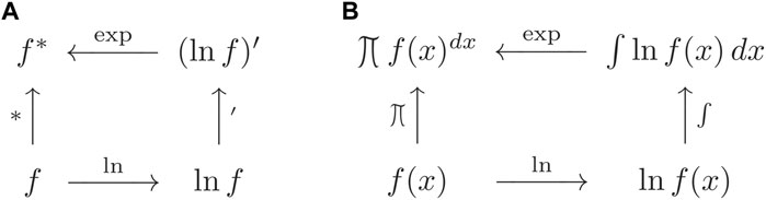
FIGURE 1. Commuting diagrams for (A) multiplicative differentiation, cf. (7) and (B) multiplicative integration, cf. (8) in terms of standard calculus counterparts via the log-exp route in the commutative case. The (upward left) operators ∗ and ∏ are defined by virtue of the equivalent counterclockwise “classical” routes in these diagrams.

The multiplicative antiderivative is then naturally defined as

$\mathit{\prod }f{\left(x\right)}^{dx}\doteq \exp (\int \ln f\left(x\right)dx).(8)$

The left hand side notation is due to Gill (Gill and Johansen, 1990) in analogy with Leibiz “continuous-sum” symbol.

For a product antiderivative or indefinite product integral we have

$\prod f{\left(x\right)}^{dx}=cF\left(x\right)\text{for\hspace{0.17em}some\hspace{0.17em}constant}c\in {\mathbb{R}}^{+}\text{iff}{F}^{*}=f,(9)$

mimicking its familiar standard counterpart

$\int f\left(x\right)dx=F\left(x\right)+c\text{for\hspace{0.17em}some\hspace{0.17em}constant\hspace{0.17em}\hspace{0.17em}}c\in \mathbb{R}\text{iff}{F}^{\prime }=f.(10)$

Definite product integrals are introduced via a spatial partitioning and limiting procedure,

$\prod _a^{b}f{\left(x\right)}^{dx}=\underset{△x_i\to 0}{\lim }\prod _{i=1}^{N}f{\left({\xi }_i\right)}^{△x_i},(11)$

akin to the standard Riemann sum approximation in the additive case,

${\int }_a^{b}f\left(x\right)dx=\underset{△x_i\to 0}{\lim }\sum _{i=1}^{N}f\left({\xi }_i\right)△x_i,(12)$

in which △x_i = x_i − x_{i − 1}, ξ_i ∈ (x_i−1, x_i) and x₀ = a, x_N = b. The relationship between Eq. 9, and Eq. 11 is formalized by the fundamental theorem of multiplicative calculus:

$\prod _a^b{F}^{*}{\left(x\right)}^{dx}=\frac{F\left(b\right)}{F\left(a\right)},(13)$

recall the well-known classical counterpart relating Eq. 10 and Eq. 12:

${\int }_a^b{F}^{\prime }\left(x\right)dx=F\left(b\right)-F\left(a\right).(14)$

Numerical approximations of Eq. 11 are obtained by partitioning the integration domain and suppressing the limiting procedure.

It requires minor efforts to generalize foregoing results to the multivariate case. The non-commutative case, on the other hand, is highly nontrivial and not without ambiguity. The complication is apparent from the ambiguous ordering of non-commuting factors on the right hand side of Eq. 11. There are multiple options to establish an unambiguous definition, cf. Gantmacher (2001) and Slavík (2007)) We will briefly discuss some and subsequently pick the one suited for our purpose.

The log-exp framework may seem the most straightforward option, defining the multiplicative derivative of a positive symmetric matrix function according to Eq. 7, in which log and exp are replaced by their well-defined matrix counterparts. The chain rule for matrix functions, however, complicates matters. Declining from the assumption of commutativity we have, e.g.

${\left(\exp g\left(x\right)\right)}^{\prime }={\int }_0^1\exp \left(\alpha g\left(x\right)\right)g^{\prime }\left(x\right)\exp \left(\left(1-\alpha \right)g\left(x\right)\right)d\alpha ,(15)$

for an arbitrary (square) matrix field g. For a positive symmetric matrix field f we furthermore have

${\left(\ln f\left(x\right)\right)}^{\prime }={\int }_0^1{\left(\alpha f\left(x\right)+\left(1-\alpha \right)I\right)}^{-1}{f}^{\prime }\left(x\right){\left(\alpha f\left(x\right)+\left(1-\alpha \right)I\right)}^{-1}d\alpha ,(16)$

in which I is the identity matrix. Both identities can be readily proven with the help of the defining Taylor series expansions of the exp and ln functions, cf. Higham (2008). In the commutative case (only) Eqs 15 and 16 reproduce the familiar chain rule formulas

${\left(\exp g\left(x\right)\right)}^{\prime }=g^{\prime }\left(x\right)\exp g\left(x\right)=\exp g\left(x\right)g^{\prime }\left(x\right),(17)$

and

${\left(\ln f\left(x\right)\right)}^{\prime }=f^{\prime }\left(x\right)f{\left(x\right)}^{-1}=f{\left(x\right)}^{-1}{f}^{\prime }\left(x\right),(18)$

well-known from classical calculus. In view of this one may avoid the cumbersome expression of Eq. 16 resulting from the log-exp trick of Eq. 7 by defining the multiplicative derivative in a different way, viz. by replacing the expression (ln f(x))′ on the right hand side in Eq. 7 formally by one of the alternative expressions in Eq. 18. As these two options (or any alternative construct obtained by sandwiching factorizations of f(x)⁻¹ = f(x)^{α − 1} f(x)^−α around f′(x)) are clearly different, the application context should determine one’s bias. We will adhere to the following definition:

$f^{*}\left(x\right)\doteq \exp \left(f^{\prime }\left(x\right)f^{-1}\left(x\right)\right).(19)$

It can be shown that, with this choice, Eq. 11 is applicable, provided we use a right-to-left ordering of factors on the right hand side:

$\prod _a^{b}f{\left(x\right)}^{dx}=\underset{△x_i\to 0}{\lim }f{\left({\xi }_N\right)}^{△x_N}\dots ,f{\left({\xi }_1\right)}^{△x_1}.(20)$

The reason for choosing Eqs 19 and 20 is that these provide the correct derivative/antiderivative for recasting a linear matrix differential equation f′ = A f, with positivity constraint on f—which will be of interest later, notably in Eq. 48 on page 13—, into its natural multiplicative counterpart with built-in positivity preservation, viz. f* = exp A. The solution then takes the trivial form of an antiderivative, $f\left(x\right)=\prod exp\left(A\right(x\left)\mathrm{dx}\right)$, according to³ Eq. 20.

Another application of multiplicative calculus relevant for our purpose is the so-called log-Euclidean paradigm for symmetric positive-definite matrix functions⁴ (Arsigny et al., 2006; Fillard et al., 2007; Pennec et al., 2006). We consider it in the context of multiscale representations (Florack and Astola, 2008). Figure 2 shows how to construct a consistent multiscale representation f_t of a raw symmetric postive-definite matrix function f ≐ f₀, with t > 0 denoting (quadratic) scale, according to the following multiplicative convolution recipe:

$f_t=\exp \left({\varphi }_t\ast \ln f\right),(21)$

in which ϕ_t denotes the normalized isotropic Gaussian of (quadratic) scale t and ∗ acts component-wise:

${\varphi }_t\left(x\right)\doteq \frac{1}{{\sqrt{4\pi t}}^n}\exp \left(-\frac{\Vert x{\Vert }^2}{4t}\right).(22)$

FIGURE 2

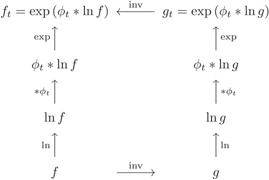
FIGURE 2. Commuting diagram for blurring and inversion. The diagram shows that inverse relationships are preserved under blurring, so that we may arbitrarily alter data resolution in any of the dual domains of definition of either f or f ^inv as per (21).

This scheme ensures closure and commutativity of blurring and inversion: If $f_t\doteq \exp \left({\varphi }_t\ast \ln f\right)$ and $g_t\doteq \exp \left({\varphi }_t\ast \ln g\right)$, with g = f⁻¹, then $g_t=f_t^{-1}$ at all scales t > 0.

2.3 Riemann-Finsler Geometry

Riemann-Finsler geometry is a generalization of Riemannian geometry. Both are metric geometries, concerned with spaces endowed with a distance concept. The generalization entails the replacement of an inner product induced norm (square root of a quadratic form reflecting the Pythagorean rule) by a general norm. For this reason Riemann-Finsler geometry is sometimes referred to as ‘Riemannian geometry without the quadratic restriction’. First studied by Finsler (1918), it has matured towards its present form mainly due to Cartan (1934). The mathematics is rather mind-boggling. For modern in-depth accounts cf. Bao et al. (2000), Shen and Shen (2016), and Antonelli et al. (1993); (Antonelli and Zastawniak, 1999) in relation to some applications in physics and biology. Riemann-Finsler geometry is also attracting considerable attention in the context of (quantum) gravity, see for example (Fuster and Pabst, 2016; Gibbons et al., 2007; Girelli et al., 2007; Pfeifer and Wohlfarth, 2012).

For our purpose a norm is needed to introduce an abstract notion of “length” of a curve, one for which units of length are proportional to local mean free path lengths of diffusing water molecules in the underlying fibrous tissue, as observed via DWI. This implies that if local mean free paths are indeed longest along biological tracts, then such tracts would define “locally shortest” paths, or geodesics, along a Riemann-Finsler manifold. The attribute “local” means that any sufficiently small perturbation of a fiducial geodesic with fixed endpoints would incur an increase of length. This leaves room for multiple geodesics connecting the same pair of endpoints. The Hopf-Rinow theorem (Jost, 2011) ensures geodesic completeness, i.e. the existence of a “minimal geodesic”, the length of which corresponds to (or, if you want, defines) the distance between its endpoints. In the case of multiple local minima between two endpoints, the global one is not necessarily the biologically most plausible one.

The Riemann-Finsler manifold is thus constructed in order to turn the tractography problem into a geodesic problem, which falls within the scope of the calculus of variations, recall section 2.1. The inherently positive nature of distance naturally calls for multiplicative calculus, recall section 2.2.

The most general functional expressing the Riemann-Finsler length of a tentative tract, arbitrarily parametrized as x = x(t), has the following form, recall Eq. 4:

$S\left(x\right)\doteq {\int }_{I\subset \mathbb{R}}F\left(x\left(t\right),\dot{x}\left(t\right)\right)dt,(23)$

in which the general Lagrangian $L(t,x,\dot{x})$ has been replaced by the so-called Finsler norm $F(x,\dot{x})$, expressing the Riemann-Finsler length of the tangent vector $\dot{x}$ at point x in a parameter invariant way. The latter not only means that it does not explicitly depend on the curve parameter t ∈ I, but also that it must be absolutely homogeneous of degree one, i.e.⁵

$F\left(x,\lambda \dot{x}\right)=|\lambda |F\left(x,\dot{x}\right),(24)$

for any tangent vector rescaling by $\lambda \in \mathbb{R}$.

One can show that, under mild conditions besides Eq. 24, there exists a positive-definite symmetric Riemann-Finsler metric tensor $g_{ij}(x,\dot{x})$, such that⁶

$F\left(x,\dot{x}\right)=\sqrt{g_{ij}\left(x,\dot{x}\right){\dot{x}}^i{\dot{x}}^j}.(25)$

The relation between $F(x,\dot{x})$ and $g_{ij}(x,\dot{x})$ is, remarkably, one-to-one, with

$g_{ij}\left(x,\dot{x}\right)=\frac{1}{2}\frac{{\partial }^2{F}^2\left(x,\dot{x}\right)}{\partial {\dot{x}}^i\partial {\dot{x}}^j}.(26)$

The Riemann-Finsler metric tensor is homogeneous of degree zero,

$g_{ij}\left(x,\lambda \dot{x}\right)=g_{ij}\left(x,\dot{x}\right).(27)$

Thus a Riemann-Finsler metric has an orientation dependency, but magnitude and “polarity” of the tangent vector $\dot{x}$ are immaterial.

The quadratic restriction of Riemannian geometry entails a severe restriction on the Finsler norm, viz. $g_{ij}(x,\dot{x})=g_{ij}(x)$ independent of orientation. Equation 26 may be interpreted as a family of Riemannian metrics, one for each orientation. All members of this family clearly coincide in the Riemannian case, so that Eq. 25 reduces to its Riemannian counterpart, the Pythagorean form

$F\left(x,\dot{x}\right)=\sqrt{g_{ij}\left(x\right){\dot{x}}^i{\dot{x}}^j}.(28)$

The Euler-Lagrange equations for Eq. 25 are known as the geodesic equations, and take the form

${\ddot{x}}^i\left(t\right)+G^i\left(x\left(t\right),\dot{x}\left(t\right)\right)=\frac{d\ln F\left(x\left(t\right),\dot{x}\left(t\right)\right)}{dt}{\dot{x}}^i\left(t\right).(29)$

The right hand side can be seen as a pseudoforce acting along the geodesic and as such merely reflects the arbitrariness of “time”-parametrization, contributing to an artificial acceleration along the trajectory. It has no effect on the relevant (parameter-invariant) geometry of the curve and can be effectively removed via (nonlinear) reparametrization. Any new parameter thus obtained is then coined an affine parameter, yielding “constant speed” geodesics characterized by $F(x(t),\dot{x}(t))=\text{constant}$. The geodesic spray coefficients $G^i(x(t),\dot{x}(t))$ can be viewed as forces inducing an acceleration and bending of the trajectory that is completely determined by the inhomogeneous nature of the metric tensor, cf. Bao (Bao et al., 2000) or Shen and Shen Shen and Shen (2016) for technical details. In the Riemannian limit they assume a quadratic form in the velocities $\dot{x}$.

Figure 3 illustrates the rationale of constructing the action functional Eq. 23 as a data-induced curve length in the context of the variational principle for the Riemannian case applicable to DTI.

FIGURE 3

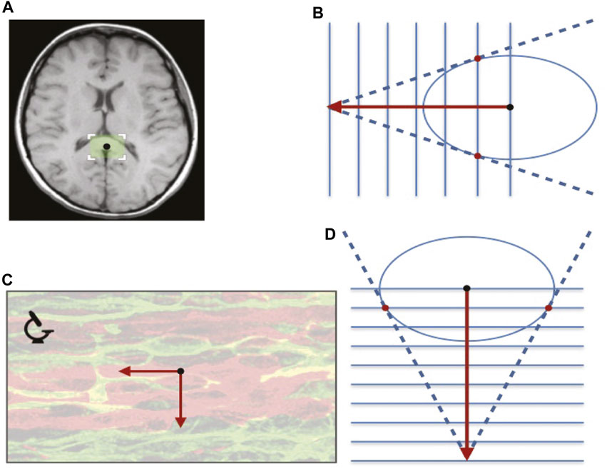
FIGURE 3. Riemann-DTI paradigm. At a typical point x inside the corpus callosum (black dot in the ROI in the MRI slice) there is a neat alignment of axons (cf. the microscopy image), inducing a diffusion tensor stretched along the preferred orientation as depicted on the right. The ellipsoid is a graphical representation of the quadratic form induced by the Riemannian metric, showing the unit level set g_ij(x)yⁱy^j = 1 for fixed x, with g_ij(x) identified with the (i, j)-th entry of the inverse diffusion tensor. The red arrows illustrate two local tangent vectors. The horizontal one aligns well with the preferred orientation, rendering its Riemannian length relatively short (upper right) as compared to the vertical one of the same Euclidean length (lower right). Geometrically, this length can be inferred via the stack of parallel planes, illustrating the corresponding dual covectors constructed on the basis of the metric via the tangent cone drawn from the tip of each vector to the ellipsoid. In this case one reads off a vector’s squared Riemannian length by counting the number of intervals spanned by it: 6, respectively nine for the horizontal and vertical arrows. Note that from a Riemann-intrinsic point of view, i.e. without reference to Euclidean concepts (such as the rigid rotation relating the two arrows), no preferred orientation can be determined. After all, the ellipsoid is, by definition, the Riemannian unit sphere, intended to mask the anisotropic nature of the underlying tissue altogether!

Apart from the geodesic equations, Eq. 29, we will be interested in “tidal effects’, i.e. the relative separation acceleration⁷ of neighbouring geodesics, aka geodesic deviation. This is relevant for understanding how stable a geodesic is with respect to small perturbations. By quantifying this one can analytically predict (to linear approximation) the behaviour of sufficiently narrow bundles of geodesics around any fiducial geodesic. Understanding geodesic deviation in a general metric space requires some fairly sophisticated mathematical machinery. It suffices here to convey the gist of it.

The geodesic deviation equations form a linear system of ordinary differential equations for a deviation vector ξ = ξ(t) defined along a given geodesic curve x = x(t). This vector can be seen as connecting points on two ‘infinitesimally’ neighbouring geodesics at the same parameter value t (one must, to begin with, first agree on an unambiguous affine parametrization). We have

$\frac{{\delta }^2{\xi }^i\left(t\right)}{\delta t^2}+{\mathrm{K}}_{jk\ell }^i\left(x\left(t\right),\dot{x}\left(t\right)\right){\dot{x}}^j\left(t\right){\dot{x}}^k\left(t\right){\xi }^{\ell }\left(t\right)=0.(30)$

The δ-derivative is a so-called covariant modification of the d-derivative from standard calculus, involving geometric ‘correction terms’ that depend on partial derivatives of the metric tensor $g_{ij}(x,\dot{x})$ with respect to both variables. The tensor field ${\mathrm{K}}_{jk\ell }^i(x,\dot{x})$ is one of the curvature tensors that can be defined on a Finsler manifold. In the Riemannian case Eq. 30 simplifies considerably, with ${\mathrm{K}}_{jk\ell }^i(x,\dot{x})$ reducing to the so-called Riemann curvature tensor ${\text{R}}_{jk\ell }^i(x)$ (a function of x only). In the particular case of interest, with n = 3 spatial dimensions, it may be reduced further to involve only the symmetric Ricci tensor field R_ij (x), with six local degrees of freedom

${\mathrm{R}}_{ij}\left(x\right)={\mathrm{R}}_{ikj}^k\left(x\right)(31)$

The interested reader is referred to the literature for technical details (Bao et al., 2000; Shen and Shen, 2016; Rund, 1959).

2.4 Riemann-DTI Paradigm: Geodesic Tractography

DTI tensors are represented by symmetric positive definite matrices obtained by fitting their six degrees of freedom at a fiducial point x to the DWI local signal attenuation factor according to the anisotropic Stejskal-Tanner equation (Stejskal and Tanner (1965); Stejskal (1965)),

$E\left(x,q\right)=\exp \left(-b{D}^{ij}\left(x\right)q_i{q}_j\right),(32)$

in which q denotes the diffusion sensitizing magnetic gradient direction⁸ and b a dimensionful constant related to diffusion time and gradient magnitude used in the scanning protocol. A Riemannian metric may then be constructed proportional to the inverse of the DTI tensor (O’Donnell et al., 2002; Lenglet et al., 2004; Fuster et al., 2016)

$g_{ij}\left(x\right)\propto D_{ij}^{\text{inv}}\left(x\right).(33)$

The metric tensor is now only dependent on the position x and not on the orientation $\dot{x}$, so that the Riemannian length of a parameterized curve x = x(t) is given by

$S\left(x\right)={\int }_{I\subset \mathbb{R}}\sqrt{g_{ij}\left(x\right){\dot{x}}^i{\dot{x}}^j}dt,(34)$

recall Eqs 23, 28. Recall that geodesic tractography entails finding curves x = x(t) for which S(x) is locally minimal. This endeavour may be tackled in two different ways, either by directly minimizing Eq. 34, or by solving its Euler-Lagrange equations, Eq. 29. In the Riemannian case at hand, and using an affine (“constant speed”) parametrization, these equations reduce to

${\ddot{x}}^i\left(t\right)+{\mathrm{\Gamma }}_{jk}^i\left(x\left(t\right)\right){\dot{x}}^j\left(t\right){\dot{x}}^k\left(t\right)=0,(35)$

in which the so-called Christoffel symbols of the second kind (Spivak, 1975) are given by linear combinations of derivatives of g_ij:

${\mathrm{\Gamma }}_{jk}^i\left(x\right)=\frac{1}{2}{g}^{im}\left(x\right)\left({\partial }_j{g}_{km}\left(x\right)+{\partial }_k{g}_{mj}\left(x\right)-{\partial }_m{g}_{jk}\left(x\right)\right).(36)$

Equation 35 may be reformulated in purely geometrical terms by defining a so-called covariant differential operator D (Spivak, 1975), given in terms of the standard differential operator d and Γ-correction terms (a special case of the δ-operator used in Eq. 30), accounting for the non-constant nature of g_ij (x). For a vector function v = v (t) defined along the curve x = x (t) we have

$\frac{D{v}^i\left(t\right)}{dt}=\frac{d{v}^i\left(t\right)}{dt}+{\mathrm{\Gamma }}_{jk}^i\left(x\left(t\right)\right)v^j\left(t\right){\dot{x}}^k\left(t\right),(37)$

so that Eq. 35 is equivalent to

$\frac{D{\dot{x}}^i\left(t\right)}{dt}=0.(38)$

For disambiguation of its solution, Eq. 35 requires a pair of initial or boundary conditions

$\left(x\left(0\right),\dot{x}\left(0\right)\right)\doteq \left(x_0,v_0\right),\text{or}(\mathrm{39a})$

$\left(x\left(0\right),x\left(T\right)\right)\doteq \left(x_0,x_T\right).(\mathrm{39b})$

The existence of a geodesic constrained by either Eq. 39a or 39b is guaranteed by the Hopf-Rinow theorem (Jost, 2011). For this reason the x-manifold is called geodesically complete. Uniqueness is not provided for the boundary problem, as there may be multiple curves (locally) minimizing Eq. 34 for sufficiently distant endpoints x₀ and x_T allowing for multiple potential fiber tracts connecting these endpoints.

2.5 Riemann-DTI Paradigm: Geodesic Deviation

Let us consider a single geodesic x = x (t) obtained either by minimization of Eq. 34 or by integration of Eq. 35. In order to understand the stability of this geodesic with respect to small perturbations of its initial or boundary conditions, Eq. 39, we may employ perturbation theory in the form of the linear geodesic deviation equations, recall Eq. 30, restricted to the Riemannian case of interest. This allows us to predict the behaviour of neighbouring geodesics without explicitly solving their nonlinear geodesic equations, as long as these are sufficiently close to the fiducial geodesic x = x (t), as described in Sengers et al. (2021), in which families of neighbouring geodesics are defined via continuous perturbations of the side conditions, Eq. 39. Here we extend our uncertainty quantification by including the effect of DTI data noise, i.e. perturbations of the metric field g_ij (x) along (a full neighbourhood of) a fiducial geodesic, which requires a generalization of Eq. 30 by accounting for an inhomogeneous “force” term. We consider general perturbations of the metric field, as to capture the intrinsic data-induced uncertainty, arising when using the Riemann-DTI tractography paradigm. In practice, these perturbations include perturbations in the DTI tensor and the underlying DWI data.

Thus we consider two types of perturbations, those affecting the intitial or boundary conditions in Eq. 39 and those affecting the metric field, viz.

$\left({\bar{x}}_0,{\bar{v}}_0\right)=\left(x_0,v_0\right)+\epsilon \left(y_0,w_0\right)+\mathcal{O}\left({\epsilon }^2\right),(\mathrm{40a})$

$\left({\bar{x}}_0,{\bar{x}}_T\right)=\left(x_0,x_T\right)+\epsilon \left(y_0,y_T\right)+\mathcal{O}\left({\epsilon }^2\right),(\mathrm{40b})$

respectively

${\bar{g}}_{ij}\left(x;\epsilon \right)=g_{ij}\left(x\right)+\epsilon h_{ij}\left(x\right)+\mathcal{O}\left({\epsilon }^2\right).(41)$

The formal parameter 0 ≤ ɛ≪ 1 is dimensionless. We are interested in $\mathcal{O}(\epsilon )$ effects; $\mathcal{O}({\epsilon }^2)$ terms are considered irrelevant and will be suppressed⁹.

For an arbitrary geodesic x = x (t) satisfying Eq. 35, consider the parameterized family of neighbouring tracks,

${\bar{x}}^i\left(t;\epsilon \right)=x^i\left(t\right)+\epsilon y^i\left(t\right),(42)$

induced by any of the perturbations in Eqs 40a, 40b, 41. The perturbative, vector-valued function y = y (t), defined along the geodesic x (t), must be such that the perturbed path represents itself a geodesic with respect to the metric ${\bar{g}}_{ij}(x;\epsilon )$ for any sufficiently small value of ɛ. Thus the perturbed path, Eq. 42, satisfies Eq. 35 up to $\mathcal{O}(\epsilon )$, with the replacement $g_{ij}\to {\bar{g}}_{ij}$. The vectors y(t) are referred to as deviation vectors, measuring the extent to which $\bar{x}(t;\epsilon )$ deviates from $x(t)=\bar{x}(t;0)$. Substitution of (42) into Eq. 35, with $g_{ij}\to {\bar{g}}_{ij}$, yields (cf. Eq. 30)

$\frac{D^2{y}^i}{d{t}^2}+{\mathrm{R}}_{jk\ell }^i{\dot{x}}^j{y}^k{\dot{x}}^{\ell }=f^i,(43)$

where D/dt denotes the covariant derivative operator along x (t), recall Eq. 37, and ${\mathrm{R}}_{jk\ell }^i(x)$ is the Riemann curvature tensor given, in terms of the Christoffel symbols of Eq. 36, by

${\mathrm{R}}_{jk\ell }^i={\partial }_k{\mathrm{\Gamma }}_{j\ell }^i-{\partial }_{\ell }{\mathrm{\Gamma }}_{jk}^i+{\mathrm{\Gamma }}_{km}^i{\mathrm{\Gamma }}_{j\ell }^m-{\mathrm{\Gamma }}_{\ell m}^i{\mathrm{\Gamma }}_{jk}^m.(44)$

Writing the first order expansion of the Christoffel symbols as

${\bar{\mathrm{\Gamma }}}_{jk}^i\left(x;\epsilon \right)={\mathrm{\Gamma }}_{jk}^i\left(x\right)+\epsilon {\mathrm{H}}_{jk}^i\left(x\right)+\mathcal{O}\left({\epsilon }^2\right),(45)$

akin to Eq. 41, the inhomogeneous term in Eq. 43 is given by

$f^i=-{\mathrm{H}}_{jk}^i{\dot{x}}^j{\dot{x}}^k=-\frac{1}{2}{g}^{i\ell }\left({\partial }_k{h}_{j\ell }+{\partial }_j{h}_{\ell k}-{\partial }_{\ell }{h}_{kj}-2h_{lm}{\mathrm{\Gamma }}_{jk}^m\right){\dot{x}}^j{\dot{x}}^k.(46)$

In order to appreciate the Eqs 43–46, consider the hypothetical case of a homogeneous, noise free DTI tensor image, inducing a constant metric tensor field. In the absence of noise we have no metric perturbations, so that fⁱ = 0, while the x-independent nature of the metric also induces a vanishing Riemann tensor, ${\text{R}}_{jk\ell }^i=0$, as well as a trivial covariant derivative, D/dt = d/dt. Equation 43 then reduces to ${\ddot{y}}^i=0$, implying a linear evolution of the deviation vector along the geodesic xⁱ = xⁱ(t). Both the fiducial geodesic as well as all geodesics induced by this type of deviation are then straight paths by virtue of Eqs 35–38 and Eq. 42. This is what one would expect of a deviation vector in a flat space. In a curved space, with a nonzero Riemann tensor ${\text{R}}_{jk\ell }^i$ in Eq. 43, neighbouring geodesics may be locally attracted towards or repelled away from the fiducial one, depending on the nature of curvature. Random data noise, producing a nonzero force term fⁱ in Eq. 43, adds further jitter to the geodesic paths.

Defining the block matrix $M\in {\mathbb{R}}^{6\times 6}$ and the column vectors $F,Y\in {\mathbb{R}}^6$ by

$M\left(t\right)=\left[\begin{array}{cc}\hfill -{\mathrm{\Gamma }}_{jk}^i{\dot{x}}^k\hfill & \hfill {\delta }_j^i\hfill \\ \hfill -{\mathrm{R}}_{jk\ell }^i{\dot{x}}^j{\dot{x}}^{\ell }\hfill & \hfill -{\mathrm{\Gamma }}_{jk}^i{\dot{x}}^k\hfill \end{array}\right]F\left(t\right)=\left[\begin{array}{c}\hfill 0\hfill \\ \hfill f^i\hfill \end{array}\right],\text{and}Y\left(t\right)=\left[\begin{array}{c}\hfill y\left(t\right)\hfill \\ \hfill \dot{y}\left(t\right)\hfill \end{array}\right],(47)$

Equation 43 can be written as an inhomogeneous linear first order system of matrix differential equations

$\frac{dY\left(t\right)}{dt}=M\left(t\right)Y\left(t\right)+F\left(t\right).(48)$

This equation may be solved with non-commutative multiplicative calculus (Bashirov et al., 2008; Florack and van Assen, 2012; Gill and Johansen, 1990) using the product integral defined in Eq. 20:

$Y\left(t\right)=\prod _0^t\exp \left(M\left(s\right)ds\right)\left(Y\left(0\right)+{\int }_0^t\prod _{\sigma }^0\exp \left(-M\left(\tau \right)d\tau \right)F\left(\sigma \right)d\sigma \right).(49)$

The block structure in M, F and Y induces a similar structure in the product integrals:

$\mathrm{\Pi }\left(t\right)\stackrel{\cdot }{=}\prod _0^t\exp \left(M\left(s\right)ds\right)\stackrel{\cdot }{=}\left[\begin{array}{cc}\hfill {\mathrm{\Pi }}_{11}\left(t\right)\hfill & \hfill {\mathrm{\Pi }}_{12}\left(t\right)\hfill \\ \hfill {\mathrm{\Pi }}_{21}\left(t\right)\hfill & \hfill {\mathrm{\Pi }}_{22}\left(t\right)\hfill \end{array}\right],\text{and}(\mathrm{50a})$

${\mathrm{\Pi }}^{-1}\left(t\right)=\prod _t^0\exp \left(-M\left(s\right)ds\right)\stackrel{\cdot }{=}\left[\begin{array}{cc}\hfill {\mathrm{\Xi }}_{11}\left(t\right)\hfill & \hfill {\mathrm{\Xi }}_{12}\left(t\right)\hfill \\ \hfill {\mathrm{\Xi }}_{21}\left(t\right)\hfill & \hfill {\mathrm{\Xi }}_{22}\left(t\right)\hfill \end{array}\right],(\mathrm{50b})$

with the help of which the solution y (t) to the initial value problem may be expressed compactly as

$y\left(t\right)={\mathrm{\Pi }}_{11}\left(t\right)y_0+{\mathrm{\Pi }}_{12}\left(t\right)w_0+{\int }_0^t\mathrm{\Theta }\left(t,\sigma \right)f\left(\sigma \right)d\sigma ,(51)$

with

$\mathrm{\Theta }\left(t,\sigma \right)={\mathrm{\Pi }}_{11}\left(t\right){\mathrm{\Xi }}_{12}\left(\sigma \right)+{\mathrm{\Pi }}_{12}\left(t\right){\mathrm{\Xi }}_{22}\left(\sigma \right).(52)$

If one considers instead the boundary value problem, the initial tangent vector $\dot{y}(0)=w_0$ must be treated as an unknown and upon setting t = T can be solved for in terms of y₀, y_T and ∫Θ(T, σ) f(σ) dσ. The solution of the boundary value problem presents itself as

$\begin{array}{ll}\hfill y\left(t\right)=\left({\mathrm{\Pi }}_{11}\left(t\right)-{\mathrm{\Pi }}_{12}\left(t\right)\right.& \left.{\mathrm{\Pi }}_{12}{\left(T\right)}^{-1}{\mathrm{\Pi }}_{11}\left(T\right)\right)y_0+{\mathrm{\Pi }}_{12}\left(t\right){\mathrm{\Pi }}_{12}{\left(T\right)}^{-1}{y}_T\hfill \\ \hfill & +{\int }_0^t\mathrm{\Theta }\left(t,\sigma \right)f\left(\sigma \right)d\sigma -{\mathrm{\Pi }}_{12}\left(t\right){\mathrm{\Pi }}_{12}{\left(T\right)}^{-1}{\int }_0^T\mathrm{\Theta }\left(T,\sigma \right)f\left(\sigma \right)d\sigma .\hfill \end{array}(53)$

3 Experimental Results

So far the theory has been formulated in a continuous setting. In clinical applications of tractography we have a discretized DTI and ditto metric field. This raises the question of sub-voxel tensor field interpolation and discrete differentiation for evaluating Christoffel symbols, recall Eq. 36. These issues are simultaneously handled by using a multiscale representation of the field, Eq. 21, combined with Log-Euclidean interpolation (Arsigny et al. (2006)). For technical details, cf. Florack et al. (2021). Supplied with initial conditions (39a), we may solve for a geodesic by time-integrating Eq. 35 over a specified interval t ∈ (0, T), e.g. using the Runge-Kutta fourth order integration scheme. If instead boundary conditions (39b) are supplied, both direct minimization of Eq. 34 and a non-linear solver for Eq. 35 are viable solution strategies. Finally, we may discretize the explicit analytical solutions to obtain geodesic deviation vectors from Eq. 53.

To illustrate our perturbative approach, we perform experiments on a DWI dataset from the Human Connectome Project. In our experiments the metric tensor of our Riemann-DTI paradigm is the adjugate of the DTI matrix D, $g_{ij}=\det D{D}_{ij}^{\text{inv}}$, cf. Fuster et al. (2016). We restrict ourselves to perturbations of the metric given by Eq. 41, while keeping boundary conditions fixed, Eq. 39b i.e. we only consider the influence of perturbations on the DTI tensor field. The effect of boundary variations of type Eq. 40a have recently been considered elsewhere (Sengers et al. (2021)). These two types of perturbations are invariably present in any tractography algorithm due to DTI domain and codomain uncertainties.

We simulate DTI field perturbations ${\bar{D}}_{ij}$ from D_ij by a bootstrapping procedure (Whitcher et al., 2008). Corresponding metric perturbations are then determined as $h_{ij}={\bar{g}}_{ij}-g_{ij}$ according to Eq. 41 with ɛ = 1, recall footnote 10. Subsequently, the deviation y(t) along an arbitrary track x (t) can be determined by Eq. 53, with y (0) = y(T) = 0, resulting in a perturbed track $\bar{x}(t)=x(t)+y(t)$. Recall that, apart from discretization, Eq. 53 is an analytical result, rendering this perturbation procedure quite efficient. This data noise simulation procedure is repeated so as to obtain a large collection of perturbed tracks.

For the sake of comparison we explicitly compute, for each simulated metric perturbation ${\bar{g}}_{ij}$, the geodesic $\widehat{x}(t)$ subject to $\widehat{x}(0)=x(0)$ and $\widehat{x}(T)=x(T)$. We thus obtain two collections of tracks, viz. a set of (computationally intensive) explicitly computed geodesics $\{{\widehat{x}}_k(t)\}$, and a set of (analytical, thus computationally efficient) approximations $\{{\bar{x}}_k(t)\}$ to geodesics $\{{\widehat{x}}_k(t)\}$, where k = 1, … , N pertains to the track associated with the kth perturbed DTI field. In our experiments we take N = 100.

Figure 4 illustrates the behaviour of analytical perturbations vs. simulated geodesics. In the first case the analytically computed tracks almost completely coincide with the simulation results, while in the second case a small degree of misalignment is clearly observable. Even though the DTI perturbations are of similar order everywhere, the linear approximation of Eq. 42 apparently does not suffice in all cases, from which we may infer that the mathematical notion of a “sufficiently small” perturbation is case dependent.

FIGURE 4

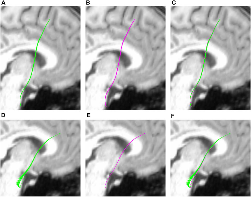
FIGURE 4. Two sets of perturbed tracks associated with two different fiducial geodesics starting in the brain stem and ending in the precentral gyrus. (A,D): In green, the collection of tracks is obtained from the analytically computed perturbations, cf. Equation 53. (B,E): In purple, tracks obtained by brute-force computation of the geodesics using the perturbed metric ${\bar{g}}_{ij}$. (C,F): Overlay for alignment comparison. The 2D background DWI image (apparent low resolution due to close-up view) is only shown for reference as a plane behind the 3D curves and it should not be used to judge the quality of the tracks. Only the difference between the analytical and simulated perturbations is of interest here.

In Figure 5 we extend the experiment of Figure 4 to a bundle of geodesics. For each of 4,237 (unperturbed) geodesics starting in the brain stem and ending in the precentral gyrus, their (simulated) perturbed geodesics $\{{\widehat{x}}_k\}$ and (analytical) approximations $\{{\bar{x}}_k\}$ are determined, again with k = 1, … , N = 100, producing two sets of 423,700 tracks each. For each of these sets we construct isosurfaces of the densities obtained by counting the number of tracks passing through each voxel. Subsequently, we threshold the density maps and construct two additional ones, so called difference maps. The difference is set to ±1 for voxels in which fibers are present in only one of the two density maps, and to 0 otherwise. A significant overlap between the analytical and simulated isosurfaces can be observed, confirming the feasibility of our approach.

FIGURE 5

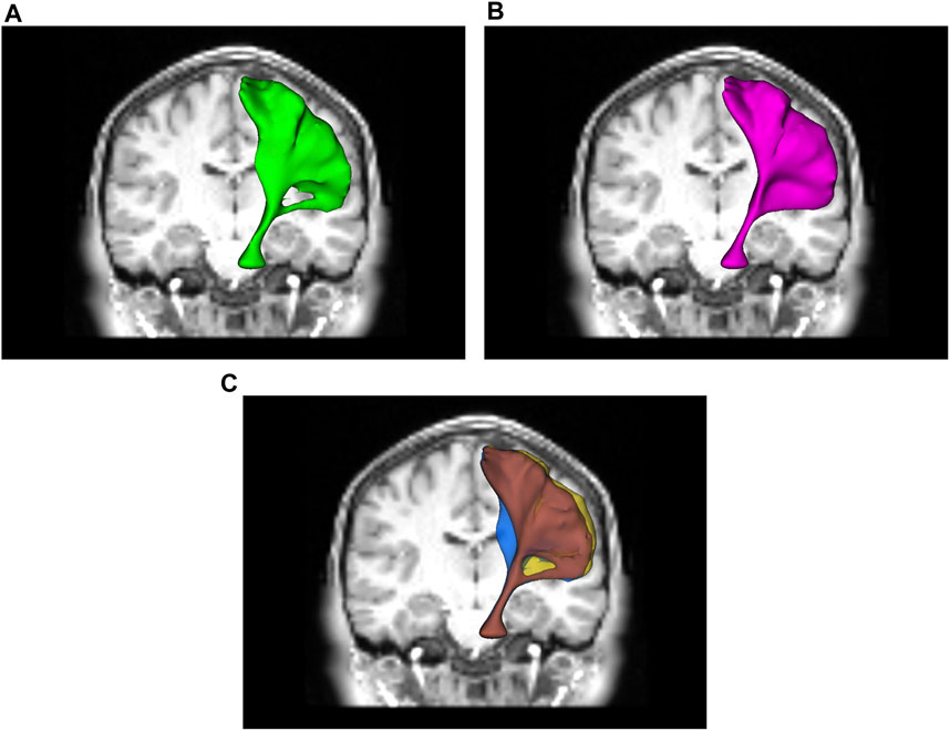
FIGURE 5. (A): The green isosurface is obtained by accumulating the analytically computed perturbations, cf. Equation 53 for 4,237 tracks. (B): The purple isosurface is obtained by recomputing the geodesics with the simulated perturbed metric ${\bar{g}}_{ij}$ for each of those 4,237 tracks. (C): The red surface contains is the intersection of the analytical (green) and simulated (purple) isosurfaces. The blue surface indicates the region which contains analytically perturbed tracks but not simulated tracks, and vice versa for the yellow surface. The background DWI image is included purely for reference to the location of the bundle in the brain. However, since the slice of the DWI image is offset from the bundle itself, this visualisation should not be used to judge the quality of the tracks, merely that of the difference between the analytically computed perturbations and their simulated counterparts.

4 Discussion

We have presented an extension to the Riemann-DTI paradigm in the form of an uncertainty quantification due to DTI data noise. To appreciate the Riemmanian framework an overview of some of the neccesary tools upon which it is built is given as well. Variational calculus lies at the basis of geodesic tractography as the mathematical machinery allowing to deduce the geodesic equations from the length functional in the form of Euler-Lagrange equations. The solutions of the geodesic equations are the locally “shortest” paths between two fiducial points in the brain, when “distance” is measured in units of mean free path length by the (inverse) of the DTI tensor.

Linear perturbation theory is applied to the geodesic equations, taking into account perturbations in the metric field induced by DTI noise, and leading to an inhomogeneous geodesic deviation equation. Together with multiplicative calculus, notably product integrals, this allow us to express the first order behaviour of the perturbations along the tracks in closed-form. As long as the perturbations in the DTI tensor are sufficiently small (which is case dependent), the analytically computed perturbed tracks do not significantly differ from the explicitly computed tracks, which are geodesics with respect to the perturbed DTI metric.

This is confirmed by our experiments, both in the case of a single (unperturbed) geodesic as well as for bundles of geodesics. In the experiments we compared both the analytically computed perturbations as well as the simulated geodesics with respect to the perturbed metric. In practice, however, one may prefer the analytical approach, as it offers a strong computational advantage. By doing brute force simulations we need to solve non-linear differential equations to find the perturbed tracks, while in our analytical approach we employ a linear differential equation with a closed-form solution that can be efficiently computed.

We recall that geodesic completeness ensures (at least) one connecting track for any pair of sufficiently distant endpoints. In case of multiple connections external knowledge may be necessary to select the most plausible one from the biological point of view. For example, tractometric features can be used to classify and subsequently prune connections according to their diffusion-related characteristics (Colby et al. (2012); De Santis et al. (2014)). We will address this important point in future work.

Our perturbative analysis may be extended past the Riemannian paradigm by using Finsler geometry, which appears to be a natural extension for general DWI models beyond DTI. This extension removes the quadratic restriction in the metric and allows for a more accurate modelling of the DWI signal capturing additional features such as intra-voxel heterogeneity, e.g. due to partial volume effects or crossing fibers. The Finslerian approach yields stronger descriptive power, at the cost of a mathematically similar but more cumbersome representation. The Finslerian counterpart of the Riemannian geodesic deviation equation may likewise inform us on the effect of perturbations on general DWI data.

Data Availability Statement

Publicly available datasets were analyzed in this study. This data can be found here: ConnectomeDB repository on https://db.humanconnectome.org; dataset “WU-Minn HCP Data—1200 Subjects”; subject 100307.

Author Contributions

RS and LF contributed equally with different emphases. Abstract and Sections 1 and 2 were written by LF. Theory outlined in Section 3 is joint work by RS and LF. Experiments described in Section 3 are conducted by RS, including algorithmic implementations. Section 4 is joint work by all authors. AF contributed to the overall setup, critical proofreading, and editorial, and to the fundamental research on which this article is based.

Funding

Data collection and sharing for this project was provided by the MGH-USC Human Connectome Project (HCP; Principal Investigators: Bruce Rosen, M.D., Ph.D., Arthur W. Toga, Ph.D., Van J. Weeden, MD). HCP funding was provided by the National Institute of Dental and Craniofacial Research (NIDCR), the National Institute of Mental Health (NIMH), and the National Institute of Neurological Disorders and Stroke (NINDS). HCP data are disseminated by the Laboratory of Neuro Imaging at the University of Southern California.

Conflict of Interest

The authors declare that the research was conducted in the absence of any commercial or financial relationships that could be construed as a potential conflict of interest.

Publisher’s Note

All claims expressed in this article are solely those of the authors and do not necessarily represent those of their affiliated organizations, or those of the publisher, the editors and the reviewers. Any product that may be evaluated in this article, or claim that may be made by its manufacturer, is not guaranteed or endorsed by the publisher.

Acknowledgments

Data collection and sharing for this project was provided by the MGH-USC Human Connectome Project (HCP; Principal Investigators: Bruce Rosen, M.D., Ph.D., Arthur W. Toga, Ph.D., Van J. Weeden, MD). We would like to thank Faizan Siddiqui for aiding us in visualizing the results of our experiments.

Footnotes

¹Many moieties other than hydrogen exhibit the same phenomenon, but their paucity in biological specimens combined with the low sensitivity of nuclear magnetic resonance makes them less suitable for imaging. Since humans are mostly water, clinical MRI scanners are therefore set up to probe water-bound hydrogen nuclei

²Parallel transport refers to spatial variability as judged from an intrinsic, geometric point of view, which typically does not coincide with the usual Euclidean (flat space) perspective. In section 2.3 this will be made more precise.

³The alternative for Eq. 19 based on the other option suggested by Eq. 18 is naturally associated with a differential equation of the form f′ = f A and would imply a reverse ordering of factors in Eq. 20.

⁴The log-Euclidean paradigm may be most naturally considered in the context of a symmetric and commutative matrix multiplication operator ◦, given by $f◦g=\exp \left(\ln f+\ln g\right)$, cf. Burgeth et al. (2007) for a more comprehensive account of alternative matrix products. We will, however, stick to standard matrix multiplication.

⁵If no parametrized path x = x(t) is involved, then $\dot{x}$ indicates an arbitrary tangent vector argument.

⁶We use Einstein summation convention throughout: Whenever an index occurs twice, once as a lower and once as an upper index, it represents a dummy summation index. Thus e.g. $g_{ij}(x,\dot{x}){\dot{x}}^i{\dot{x}}^j$ actually denotes ${\sum }_{i,j=1}^3{g}_{ij}(x,\dot{x}){\dot{x}}^i{\dot{x}}^j$.

⁷The reason for considering relative acceleration is that this captures the essential deviation from a constant relative separation velocity observed in the case of Euclidean space.

⁸The factor b may be absorbed in the tensor q_iq_j, yielding the so-called B-tensor.

⁹For “small enough” y₀, w₀, y_T, h_ij in Eqs 40a, 41 we may set ɛ = 1 without loss of generality

References

Antonelli, P. L., Ingarden, R. S., and Matsumoto, M. (1993). The Theory of Sprays and Finsler Spaces with Applications in Physics and Biology, Vol. 58 of Fundamental Theories of Physics. Dordrecht, Netherlands: Kluwer Academic Publishers.

Google Scholar

Antonelli, P. L., and Zastawniak, T. J. (1999). Fundamentals of Finslerian Diffusion with Applications, Vol. 101 of Fundamental Theories of Physics. Dordrecht, Netherlands: Kluwer Academic Publishers. doi:10.1007/978-94-011-4824-5

CrossRef Full Text | Google Scholar

Arnold, V. I. (1989). Mathematical Methods of Classical Mechanics, Vol. 60 of Graduate Texts in Mathematics. second edn. New York: Springer-Verlag.

Google Scholar

Arsigny, V., Fillard, P., Pennec, X., and Ayache, N. (2006). Log-Euclidean Metrics for Fast and Simple Calculus on Diffusion Tensors. Magn. Reson. Med. 56, 411–421. doi:10.1002/mrm.20965

PubMed Abstract | CrossRef Full Text | Google Scholar

Astola, L., and Florack, L. (2011). Finsler Geometry on Higher Order Tensor fields and Applications to High Angular Resolution Diffusion Imaging. Int. J. Comput. Vis. 92, 325–336. doi:10.1007/s11263-010-0377-z

CrossRef Full Text | Google Scholar

Astola, L. J. (2010). “Multi-Scale Riemann-Finsler Geometry: Applications to Diffusion Tensor Imaging and High Angular Resolution Diffusion Imaging,” (Eindhoven, Netherlands: Eindhoven University of Technology, Department of Mathematics and Computer Science). Ph.D. thesis.

Google Scholar

Astola, L., Jalba, A., Balmashnova, E., and Florack, L. (2011). Finsler Streamline Tracking with Single Tensor Orientation Distribution Function for High Angular Resolution Diffusion Imaging. J. Math. Imaging Vis. 41, 170–181. doi:10.1007/s10851-011-0264-4

CrossRef Full Text | Google Scholar

Bao, D., Chern, S.-S., and Shen, Z. (2000). An Introduction to Riemann-Finsler Geometry, Vol. 2000 of Graduate Texts in Mathematics. New York: Springer-Verlag.

Google Scholar

Bashirov, A. E., Kurpınar, E. M., and Özyapıcı, A. (2008). Multiplicative Calculus and its Applications. J. Math. Anal. Appl. 337, 36–48. doi:10.1016/j.jmaa.2007.03.081

CrossRef Full Text | Google Scholar

Bloch, F. (1946). Nuclear Induction. Phys. Rev. 70, 460–474. doi:10.1103/physrev.70.460

CrossRef Full Text | Google Scholar

Brown, R. W., Haacke, E. M., Cheng, Y.-C. N., Thompson, M. R., and Venkatesan, R. (2014). Magnetic Resonance Imaging: Physical Principles and Sequence Design. New York: John Wiley & Sons.

Google Scholar

Burgeth, B., Didas, S., Florack, L., and Weickert, J. (2007). A Generic Approach to Diffusion Filtering of Matrix-fields. Computing 81, 179–197. doi:10.1007/s00607-007-0248-9

CrossRef Full Text | Google Scholar

Cartan, E. (1934). Les Espaces de Finsler. Paris: Hermann.

Google Scholar

Cartan, E. (1963). Leçons sur la Géométrie des Espaces de Riemann. second edn. Paris: Gauthiers-Villars.

Google Scholar

Colby, J. B., Soderberg, L., Lebel, C., Dinov, I. D., Thompson, P. M., and Sowell, E. R. (2012). Along-tract Statistics Allow for Enhanced Tractography Analysis. NeuroImage 59, 3227–3242. doi:10.1016/j.neuroimage.2011.11.004

PubMed Abstract | CrossRef Full Text | Google Scholar

Cowan, B. (1997). Nuclear Magnetic Resonance and Relaxation. Cambridge: Cambridge University Press.

Google Scholar

De Santis, S., Drakesmith, M., Bells, S., Assaf, Y., and Jones, D. K. (2014). Why Diffusion Tensor MRI Does Well Only Some of the Time: Variance and Covariance of white Matter Tissue Microstructure Attributes in the Living Human Brain. Neuroimage 89, 35–44. doi:10.1016/j.neuroimage.2013.12.003

PubMed Abstract | CrossRef Full Text | Google Scholar

Dela Haije, T. C. J. (2017). “Geometry in Diffusion Weighted MRI,” (Eindhoven, Netherlands: Eindhoven University of Technology). Ph.D. thesis.

Google Scholar

Dela Haije, T., Savadjiev, P., Fuster, A., Schultz, R. T., Verma, R., Florack, L., et al. (2019). Structural Connectivity Analysis Using Finsler Geometry. SIAM J. Imaging Sci. 12, 551–575. doi:10.1137/18M1209428

CrossRef Full Text | Google Scholar

D. Lovelock, and H. Rund (Editors) (1988). Tensors, Differential Forms, and Variational Principles (Mineola, N.Y.: Dover Publications, Inc.).

Google Scholar

D. Lovelock, and H. Rund (Editors) (1989). Tensors, Differential Forms, and Variational Principles (Mineola, N.Y.: Dover Publications, Inc.).

Google Scholar

do Carmo, M. P. (1976). Differential Geometry of Curves and Surfaces. Mathematics: Theory & Applications. Englewood Cliffs, New Jersey: Prentice-Hall.

Google Scholar

do Carmo, M. P. (1993). Riemannian Geometry. Mathematics: Theory & Applications. second edn. Boston: Birkhäuser.

Google Scholar

Fillard, P., Pennec, X., Arsigny, V., and Ayache, N. (2007). Clinical DT-MRI Estimation, Smoothing, and Fiber Tracking with Log-Euclidean Metrics. IEEE Trans. Med. Imaging 26, 1472–1482. doi:10.1109/tmi.2007.899173

PubMed Abstract | CrossRef Full Text | Google Scholar

Finsler, P. (1918). “Ueber Kurven und Flächen in allgemeinen Räumen,” (Göttingen, Germany: University of Göttingen). Ph.D. thesis.

Google Scholar

Florack, L., Dela Haije, T., and Fuster, A. (2015). “Direction-controlled DTI Interpolation,” in Visualization and Processing of Tensors and Higher Order Descriptors for Multi-Valued Data. Mathematics and Visualization. Editors I. Hotz, and T. Schultz (Berlin, Germany: Springer-Verlag), 149–162. doi:10.1007/978-3-319-15090-1_8

CrossRef Full Text | Google Scholar

Florack, L., and Fuster, A. (2014). “Riemann-Finsler Geometry for Diffusion Weighted Magnetic Resonance Imaging,” in Visualization and Processing of Tensors and Higher Order Descriptors for Multi-Valued Data. Mathematics and Visualization. Editors C.-F. Westin, A. Vilanova, and B. Burgeth (Berlin, Germany: Springer-Verlag), 189–208. doi:10.1007/978-3-642-54301-2_8

CrossRef Full Text | Google Scholar

Florack, L. M. J., and Astola, L. J. (2008). “A Multi-Resolution Framework for Diffusion Tensor Images,” in CVPR Workshop on Tensors in Image Processing and Computer Vision, Anchorage, Alaska, USA, June 24–26, 2008. Editors S. Aja Fernández, and R. de Luis Garcia (IEEE). Digital proceedings.

CrossRef Full Text | Google Scholar

Florack, L., Sengers, R., Meesters, S., Smolders, L., and Fuster, A. (2021). “Riemann-DTI Geodesic Tractography Revisited,” in Anisotropy across Fields and Scales. Mathematics and Visualization. Editors E. Özarslan, T. Schultz, E. Zhang, and A. Fuster (Berlin, Germany: Springer-Verlag), 225–243. doi:10.1007/978-3-030-56215-1_11

CrossRef Full Text | Google Scholar

Florack, L., and van Assen, H. (2012). Multiplicative Calculus in Biomedical Image Analysis. J. Math. Imaging Vis. 42, 64–75. doi:10.1007/s10851-011-0275-1

CrossRef Full Text | Google Scholar

Fuster, A., Dela Haije, T., Tristán-Vega, A., Plantinga, B., Westin, C.-F., and Florack, L. (2016). Adjugate Diffusion Tensors for Geodesic Tractography in white Matter. J. Math. Imaging Vis. 54, 1–14. doi:10.1007/s10851-015-0586-8

CrossRef Full Text | Google Scholar

Fuster, A., and Pabst, C. (2016). Finslerpp-waves. Phys. Rev. D 94, 104072–1–104072–5. doi:10.1103/PhysRevD.94.104072

CrossRef Full Text | Google Scholar

Gantmacher, F. R. (2001). The Theory of Matrices. Providence, Rhode Island: American Mathematical Society.

Google Scholar

Gibbons, G. W., Gomis, J., and Pope, C. N. (2007). General Very Special Relativity Is Finsler Geometry. Phys. Rev. D 76, 081701. doi:10.1103/PhysRevD.76.081701

CrossRef Full Text | Google Scholar

Gill, R. D., and Johansen, S. (1990). A Survey of Product-Integration with a View toward Application in Survival Analysis. Ann. Stat. 18, 1501–1555. doi:10.1214/aos/1176347865

CrossRef Full Text | Google Scholar

Girelli, F., Liberati, S., and Sindoni, L. (2007). Planck-scale Modified Dispersion Relations and Finsler Geometry. Phys. Rev. D 75. doi:10.1103/physrevd.75.064015

CrossRef Full Text | Google Scholar

H. Sagan (Editor) (1992). Calculus of Variations (New York: Dover Publications, Inc.).

Google Scholar

Higham, N. J. (2008). Functions of Matrices: Theory and Computation. Philadelphia, PA: SIAM.

Google Scholar

Jost, J. (2011). Riemannian Geometry and Geometric Analysis. Universitext. sixth edn. Berlin: Springer-Verlag.

Google Scholar

Koenderink, J. J. (1990). Solid Shape. Cambridge: MIT Press.

Google Scholar

Lenglet, C., Deriche, R., and Faugeras, O. (2004). “Inferring white Matter Geometry from Diffusion Tensor MRI: Application to Connectivity Mapping,” in Proceedings of the Eighth European Conference on Computer Vision (Prague, Czech Republic, May 2004). Editors T. Pajdla, and J. Matas (Berlin: Springer-Verlag), 127–140. vol. 3021–3024 of Lecture Notes in Computer Science. doi:10.1007/978-3-540-24673-2_11

CrossRef Full Text | Google Scholar

Maier-Hein, K. H., Neher, P. F., Houde, J. C., Côté, M. A., Garyfallidis, E., Zhong, J., et al. (2017). The challenge of Mapping the Human Connectome Based on Diffusion Tractography. Nat. Commun. 8, 1349. doi:10.1038/s41467-017-01285-x

PubMed Abstract | CrossRef Full Text | Google Scholar

Meesters, S., Landers, M., Rutten, G.-J., and Florack, L. (2021). “Automatic Tractography for Brain Tumor Surgery: Towards Clinical Application,” in Proceedings of the ISMRM & SMRT Annual Meeting & Exhibition (online, May 15–20, 2021).

Google Scholar

Meesters, S., Rutten, G.-J., Fuster, A., and Florack, L. (2019). “Automated Tractography of Four white Matter Fascicles in Support of Brain Tumor Surgery,” in 2019 OHBM Annual Meeting, Rome, Italy, June 6–13 2019 (Rome: Organization for Human Brain Mapping). Abstract nr. Th768.

Google Scholar

Misner, C. W., Thorne, K. S., and Wheeler, J. A. (1973). Gravitation. San Francisco: Freeman.

Google Scholar

Moritani, T., Ekholm, S., and Westesson, P.-L. (2009). Diffusion-Weighted MR Imaging of the Brain. second edn. Berlin, Germany: Springer-Verlag. doi:10.1007/978-3-3540-78785-3

CrossRef Full Text | Google Scholar

Neuenschwander, D. E. (2011). Emmy Noether’s Wonderful Theorem. Baltimore: The Johns Hopkins University Press.

Google Scholar

O’Donnell, L., Haker, S., and Westin, C.-F. (2002). “New Approaches to Estimation of white Matter Connectivity in Diffusion Tensor MRI: Elliptic PDEs and Geodesics in a Tensor-Warped Space,” in Proceedings of the 5th International Conference on Medical Image Computing and Computer-Assisted Intervention—MICCAI 2002, Tokyo, Japan, September 25–28 2002. Editors T. Dohi, and R. Kikinis (Berlin, Germany: Springer-Verlag), 459–466. vol. 2488–2489 of Lecture Notes in Computer Science.

Google Scholar

Pennec, X., Fillard, P., and Ayache, N. (2006). A Riemannian Framework for Tensor Computing. Int. J. Comput. Vis. 66, 41–66. doi:10.1007/s11263-005-3222-z

CrossRef Full Text | Google Scholar

Pfeifer, C., and Wohlfarth, M. N. R. (2012). Finsler Geometric Extension of Einstein Gravity. Phys. Rev. D 85. doi:10.1103/PhysRevD.85.064009

CrossRef Full Text | Google Scholar

R. Weinstock (Editor) (1974). Calculus of Variations with Applications to Physics & Engineering (New York: Dover Publications, Inc.).

Google Scholar

Rund, H. (1959). The Differential Geometry of Finsler Spaces. Berlin, Germany: Springer-Verlag.

Google Scholar

Rund, H. (1973). The Hamilton-Jacobi Theory in the Calculus of Variations. Huntington, N.Y.: Robert E. Krieger Publishing Company.

Google Scholar

Rutten, G. J. M., Kristo, G., Pigmans, W., Peluso, J., and Verheul, H. B. (2014). Het gebruik van MR-tractografie in de dagelijkse neurochirurgische praktijk (the use of MR-tractography in daily neurosurgical practice). Tijdschrift voor Neurologie & Neurochirurgie 115, 204–211. With English abstract.

Google Scholar

Schilling, K. G., Nath, V., Hansen, C., Parvathaneni, P., Blaber, J., Gao, Y., et al. (2019). Limits to Anatomical Accuracy of Diffusion Tractography Using Modern Approaches. NeuroImage 185, 1–11. doi:10.1016/j.neuroimage.2018.10.029

PubMed Abstract | CrossRef Full Text | Google Scholar

Schilling, K. G., Petit, L., Rheault, F., Remedios, S., Pierpaoli, C., Anderson, A. W., et al. (2020). Brain Connections Derived from Diffusion MRI Tractography Can Be Highly Anatomically Accurate-If We Know where white Matter Pathways Start, where They End, and where They Do Not Go. Brain Struct. Funct. 225, 2387–2402. doi:10.1007/s00429-020-02129-z

PubMed Abstract | CrossRef Full Text | Google Scholar

Sengers, R., Florack, L., and Fuster, A. (2021). “Geodesic Tubes for Uncertainty Quantification in Diffusion MRI,”in Proceedings of the Twenty-Seventh International Conference on Information Processing in Medical Imaging–IPMI 2021, Bornholm, Denmark. Editors S. Sommer, A. Feragen, J. Schnabel, and M. Nielsen (Berlin: Springer-Verlag), 279–290. vol. 12729 of Lecture Notes in Computer Science. doi:10.1007/978-3-030-78191-0_22

CrossRef Full Text | Google Scholar

Shen, Y.-B., and Shen, Z. (2016). Introduction to Modern Finsler Geometry. Singapore: World Scientific.

Google Scholar

Slavík, A. (2007). Product Integration, its History and Applications. Prague: Matfyzpress.

Google Scholar

Spivak, M. (1975). Differential Geometry, Vol. 1–5. Berkeley: Publish or Perish.

Google Scholar

Stejskal, E. O., and Tanner, J. E. (1965). Spin Diffusion Measurements: Spin Echoes in the Presence of a Time‐Dependent Field Gradient. J. Chem. Phys. 42, 288–292. doi:10.1063/1.1695690

CrossRef Full Text | Google Scholar

Stejskal, E. O. (1965). Use of Spin Echoes in a Pulsed Magnetic‐Field Gradient to Study Anisotropic, Restricted Diffusion and Flow. J. Chem. Phys. 43, 3597–3603. doi:10.1063/1.1696526

CrossRef Full Text | Google Scholar

Szilasi, J., Lovas, R. L., and Kertész, D. C. (2014). Connections, Sprays and Finsler Structures. Singapore: World Scientific.

Google Scholar

Torrey, H. C. (1956). Bloch Equations with Diffusion Terms. Phys. Rev. 104, 563–565. doi:10.1103/physrev.104.563

CrossRef Full Text | Google Scholar

Whitcher, B., Tuch, D. S., Wisco, J. J., Sorensen, A. G., and Wang, L. (2008). Using the Wild Bootstrap to Quantify Uncertainty in Diffusion Tensor Imaging. Hum. Brain Mapp. 29, 346–362. doi:10.1002/hbm.20395

PubMed Abstract | CrossRef Full Text | Google Scholar