Internal representation of task rules by recurrent dynamics: the importance of the diversity of neural responses

Introduction

Neurons in the mammalian brain are highly heterogeneous (Soltesz, 2005; Marder and Goaillard, 2006) and show diverse responses to sensory stimuli and other events. This diversity is especially bewildering with regard to the prefrontal cortex, a brain structure that has been shown to be critically important for higher cognitive behaviors in numerous lesion (Petrides, 1982; Passingham, 1993; Murray et al., 2000), clinical (Petrides, 1985), and imaging (Boettiger and D’Esposito, 2005) studies. Indeed, single-neuron recordings from the prefrontal cortex have yielded a rich phenomenology: neurons have been found to respond to sensory stimuli and show persistent activity during working memory (Fuster and Alexander, 1971; Funahashi et al., 1989; Romo et al., 1999), reflect animals’ decisions or intended actions (Tanji and Hoshi, 2008) or rewards (Barraclough et al., 2004), and encode contexts, task rules (Wallis et al., 2001; Genovesio et al., 2005; Mansouri et al., 2006, 2007) and abstract concepts like numbers (Nieder and Miller, 2003). Typically, a single prefrontal cell is not merely responsive to a single event but shows selectivity to a combination of different aspects of the task being executed (mixed selectivity). These findings naturally pose the question: does such diversity of responses play a constructive computational role in complex cognitive tasks?

We found a computational role for the neuronal response diversity, which is directly related to the function of prefrontal cortex of actively maintaining a representation of behavioral rules (Goldman-Rakic, 1987; Miller and Cohen, 2001). This is in line with previous theoretical works that have shown that specific forms of mixed selectivity can be harnessed to perform computation such as complex sensorimotor transformations (Zipser and Andersen, 1988; Pouget and Sejnowski, 1997; Pouget and Snyder, 2000; Salinas and Abbott, 2001) and to model serial working memory (Botvinick and Watanabe, 2007) and visuomotor remapping (Salinas, 2004a) (see Discussion for more details).

Rules are prescribed guides for problem solving and flexible decision making and they vary in the degree of abstraction. Examples include conditional (arbitrary) sensorimotor associations (if red light, then stop), task rules (respond if two stimuli match), strategies for decision making (if win, stay; if lose, switch). We assumed that the rule in effect is actively maintained by a recurrent neural circuit. In particular we hypothesized that the neural correlate of a rule is a self-sustained persistent pattern of activity (see e.g., Miller and Cohen, 2001). Small perturbations of these activity patterns are damped by the interactions between neurons, so that the state of the network remains close to one of the patterns of persistent activity. Hence these patterns are stable, and they are called attractors of the neural dynamics. Attractor network models have been previously studied for associative (Hopfield, 1982) and working memory (Amit, 1989; Wang, 2001) of sensory stimuli. In these models a sensory stimulus activates one of the strongly interacting populations of neurons and the memory of stimulus identity is maintained by the persistent activity of the activated population.

Our intention was to extend these models to the most general case in which every attractor corresponds to a particular rule, as assumed in studies on specific tasks (Amit, 1988; O’Reilly and Munakata, 2000; Xing and Andersen, 2000; Loh and Deco, 2005). In particular we wanted to understand how the rule can affect our decisions, and how external events can select the rule in effect. We assumed that every event generates a driving force that steers the neural activity toward a different stable pattern. Such a pattern corresponds to a new rule and depends on both the external event and the previous rule in effect.

In such a scenario, as we will show, the absence of neurons with mixed selectivity typically compromises the possibility of constructing a neural network that can perform the task. These difficulties are almost always encountered whenever the rules for committing the course of action contain a dependence on the context. For example, they are unavoidable in the case of the Wisconsin Card Sorting Test (WCST), when the subject needs to switch from one rule to another. The next rule to be selected clearly depends not only on the instruction to switch, but also on the previous rule in effect (context). The inability to switch in a WCST is often considered as an indication of a damage of prefrontal cortex (Milner, 1963), which is a brain area with abundance of mixed selectivity (see e.g., Asaad et al., 1998; Cromer et al., 2010; Rigotti et al., 2010).

We will then show that neurons with mixed selectivity and diverse response properties not only are necessary in our scenario to perform context-dependent tasks, but they are also sufficient to solve arbitrarily complicated tasks. Mixed selectivity is readily obtained by connecting cells with random connections to both the neurons in the recurrent circuit and to the neurons representing the external events. We will show that this simple form of heterogeneity grants the neural network the ability to implement arbitrarily complicated tasks. Surprisingly, it turns out that the number of randomly connected neurons needed to implement a particular task is not much larger than the minimal number of neurons required in a carefully designed neural circuit. This number grows only linearly with the number of inner mental states encoding the rules, and the task-relevant events, despite the combinatorial explosion of possible mixed selectivity responses. The randomly connected neurons possess response properties that are more diverse than required in a minimal circuit, as they respond to both necessary and unnecessary combinations of mental states and events. Moreover, such response properties are predicted to be pre-existent and universal as they should be observable before the learning process, independently from the task to be learned. Our work suggests that the observed diversity of the neural responses plays an important computational role, both in the acquisition and the execution of tasks in which our decision or our actions depend on the context.

Results

Modeling Complex Cognitive Tasks: the General Framework

In order to model the most general rule-based behavior, we assume that subjects performing complex tasks go through a series of inner mental states, each representing an actively maintained disposition to behavior or an action that is being executed. Each state contains information about task-relevant past events and internal cognitive processes representing reactivated memories, emotions, intentions and decisions, and in general all factors that will determine or affect the current or future behavior, like the execution of motor acts. In Figure 1A we illustrate this scenario in the case of a simplified version of the Wisconsin Card Sorting Test (WCST). In a typical trial, the subject sees a sample stimulus on a screen and, after a delay, he is shown two test stimuli. He has to touch the test stimulus matching either the shape or the color of the sample, depending on the rule in effect. The subject has to determine the rule by trial and error; a reward confirms that the rule was correct, and an error signal prompts the subject to switch to the alternative rule. Every task-relevant event such as the appearance of a visual stimulus or the delivery of reward is hypothesized to induce a transition to a different mental state.

FIGURE 1

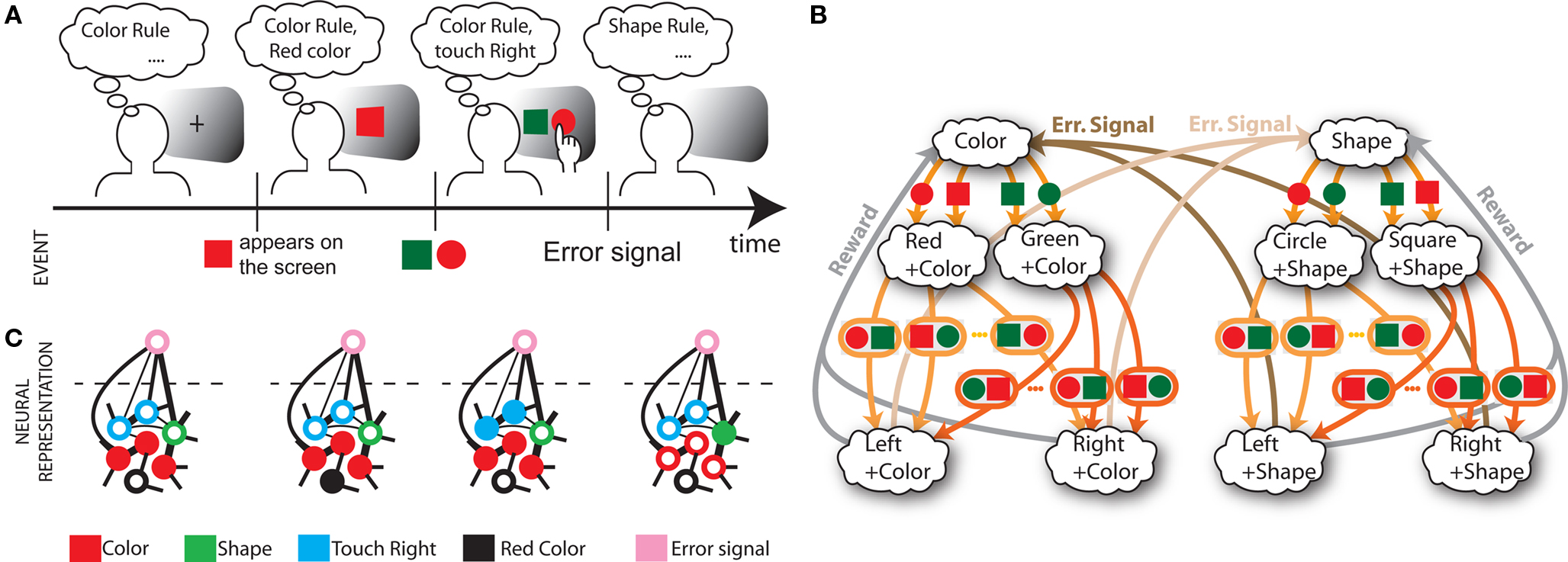
Figure 1. A context-dependent task. (A) A typical trial of a simplified version of the WCST, similar to the one used in the monkey experiment (Mansouri et al., 2006, 2007). The subject has to classify visual stimuli either according to their shape or according to their color. Before the trial starts, the subject keeps actively in mind the rule in effect (color or shape). Every event, like the appearance of a visual stimulus, modifies the mental state of the subject. An error signal indicates that it is necessary to switch to the alternative rule. (B) Scheme of mental states (thought balloons) and event-driven transitions (arrows) that enables the subject to perform the simplified WCST. (C) Neural representation of the mental states shown in (A): circles represent neurons, and colors denote their response preferences (e.g., red units respond when Color Rule is in effect). Filled circles are active neurons and black lines are synaptic connections. For simplicity, not all neurons and synaptic connections are drawn.

The neural correlate of a mental state is assumed to be a stable pattern of activity of a recurrent neural circuit. The same neural circuit can sustain multiple stable patterns corresponding to different mental states. Events like sensory stimuli, reward delivery, or error signals steer the neural activity toward a different stable pattern representing a new mental state. Such a pattern will in general depend on both the external event and the previous mental state.

In order to construct an attractor network that is able to perform a certain context-dependent task we need to find the synaptic couplings between neurons that satisfy the mathematical conditions for guaranteeing that the attractors are stable fixed points of the neural dynamics and that external events induce the desired transitions. Interestingly, we found that even in the example of very simple context-dependent motor tasks, these conditions cannot be fulfilled simultaneously, similarly to what happens in the case of semantic networks (Hinton, 1981). We will show that this is a general problem of all context-dependent tasks.

Fundamental Difficulties in Context-Dependent Tasks

To illustrate the problem caused by context dependence, consider a task switching induced by an error signal in the simplified WCST (see Figure 2A). In one context, e.g., when the Color Rule is in effect, the error signal induces a transition to the Shape Rule state at the top of the scheme of Figure 1B, whereas in the other, when starting from the Shape Rule, the same event determines the selection of the Color Rule state. In the first context the neurons of the recurrent circuit excite each other so as to sustain the pattern of persistent activity representing the Color Rule mental state. The overall recurrent input to neurons selective for Color Rule must therefore be excitatory enough to sustain the persistent activity state representing the Color Rule. On the other hand, in the Shape Rule state the overall current should be below the activation threshold (Figure 2A, left). In order to induce a rule switch, the additional synaptic input generated by the Error Signal should be inhibitory enough to overcome the recurrent input and inactivate these neurons when starting from the Color Rule mental state, and excitatory enough to activate them when starting from the Shape Rule state (Figure 2A, right). This is impossible to realize because the neural representation of the Error Signal is the same in the two contexts. This problem is equivalent to the known problem of non-linear separability of the Boolean operation of exclusive OR (XOR) and it plagues most neural networks implementing context-dependent tasks.

FIGURE 2

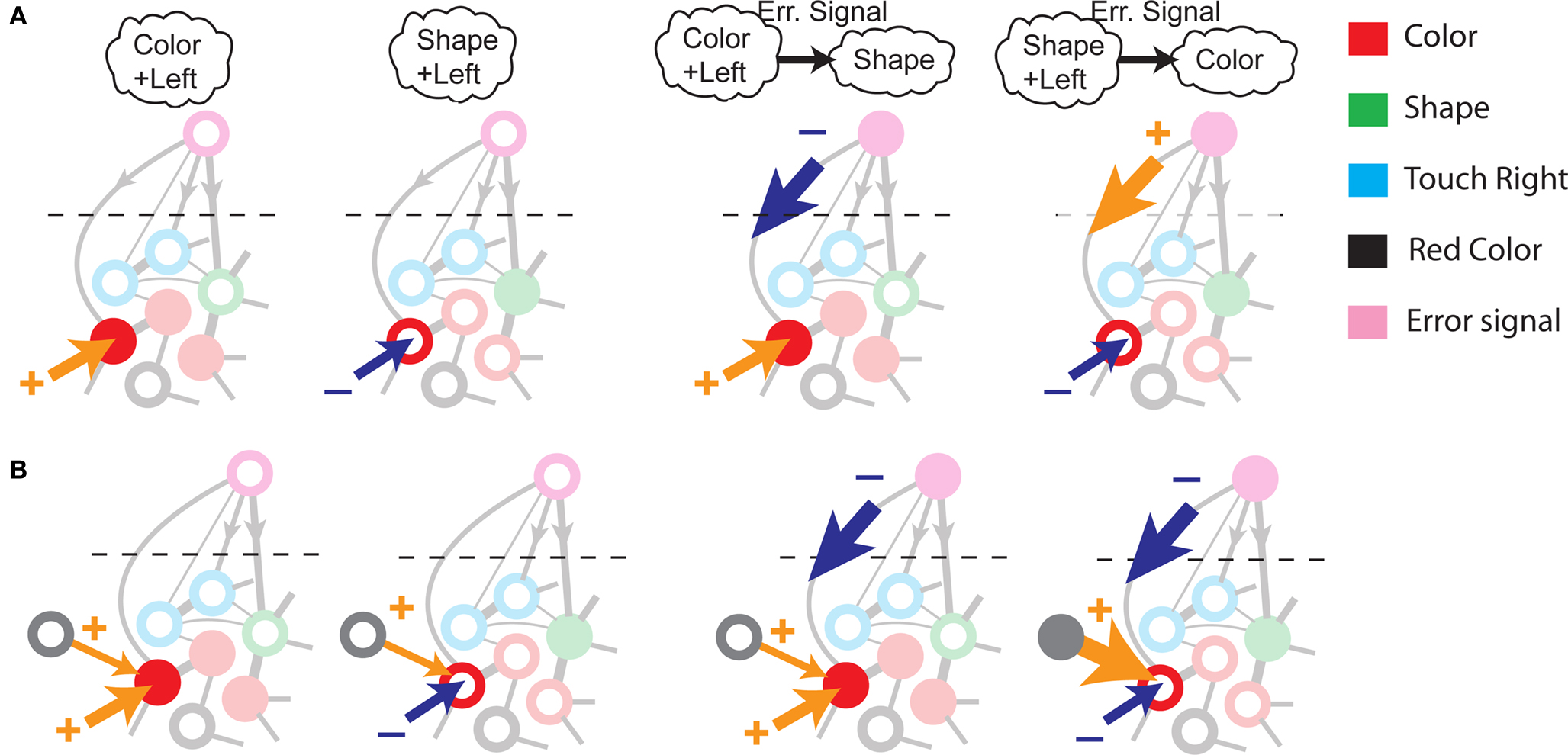
Figure 2. (A) Impossibility of implementing a context-dependent task in the absence of mixed selectivity neurons. We focus on one neuron encoding Color Rule (red). In the attractors (two panels on the left), the total recurrent synaptic current (arrow) should be excitatory when the Color Rule neuron is active, inhibitory otherwise. In case of rule switching (two panels on the right), generated by the Error Signal neuron (pink), there is a problem as the same external input should be inhibitory (dark blue) when starting from Color Rule and excitatory (orange) otherwise. (B) The effect of an additional neuron with mixed selectivity that responds to the Error Signal only when starting from Shape Rule. Its activity does not affect the attractors (two panels on the left), but it excites Color Rule neurons when switching from Shape Rule upon an Error Signal. In the presence of the mixed selectivity neurons, the current generated by the Error Signal can be chosen to be consistently inhibitory.

We illustrated the problem in a specific and schematic example, but more in general, a non-linear separability manifests itself whenever the same external event must activate a neural population in one context, and inactivate it in another, like a flip-flop. More formally, consider two attractors given by the activity patterns and (Color + Left and Shape + Left of the example of Figure 2). These represent two mental states preceding a particular event E that will induce a transition to (Shape in the example) when starting from , and to a different pattern (Color) when starting from (E = Err. Signal in Figure 2). We need to impose the following two conditions to guarantee that the mental states are fixed points of the dynamics:

where E⁰ denotes the absence of any event (e.g., when the recurrent network receives only spontaneous activity). At the same time we need to impose the two conditions corresponding to the event-driven transitions:

where E represents the external event. We now prove that there is no set of synaptic weights that satisfies all the four conditions when for some neuron i we have that

We define as (μ = 1,2) the total synaptic current to neuron i when the network is in one of the initial attractors . For simplicity and without loss of generality, we assume that the external current in the absence of events is 0. We now consider a case in which the activity of neuron i is different in the two initial mental states (i.e., when , where θ is the threshold for neuronal activation). When the external input is activated upon the occurrence of an event, an extra current H_i is injected into neuron i. The current is uniquely determined by the event and by the weights of the synapses connecting the external to the recurrent neurons. As a consequence it is the same for all initial mental states, that is for both attractors and . We can now show that in the case in which the external event should modify the activation of neuron i in both attractors, it is impossible to impose all conditions simultaneously. Indeed, consider, without loss of generality, a case in which for the attractors we have and . We also assume that the transitions require that starting from mental state 1, the neuron is inactivated (), whereas starting from mental state 2 the neuron is activated (). We see that it is not possible to fulfill all these requirements simultaneously as H_i should be negative enough to satisfy the condition for the first transition [H_i < −(I_i − θ) with I_i − θ > 0, to satisfy the mental state stationarity condition], and, at the same time, positive enough to allow for the second transition. As the synaptic currents are determined by the given patterns of neural activity and by the synaptic weights, this result implies that there is no set of synaptic weights that can satisfy all conditions. Notice that this result does not depend on the specific representations of the mental states and external events, but only on the existence of neurons whose state is activated in one context and inactivated in another context by the same event (see Section “Constraints on the Types of Implementable Context-Dependent Transitions” in Appendix for a geometrical representation of this problem).

The probability of not encountering such a problem decreases exponentially with the number of transitions and with the number of neurons in the network, if the patterns of activities representing the mental states are random and uncorrelated (see Section “Constraints on the Types of Implementable Context-Dependent Transitions” in Appendix). This result indicates that it is very likely to encounter this problem every time our action or, more in general, our next mental state, depends on the context. We will show in the next sections that neurons with mixed selectivity solve the problem in the most general case and for any neural representation.

The Importance of Mixed Selectivity

The main problem of the example illustrated in Figure 2A is originated by the assumption that each neuron is selective either to the inner mental state (Color or Shape Rule) or to the external input (such as the Error Signal). Indeed, consider an additional neuron that responds to the Error Signal only when the neural circuit is in the state corresponding to the Shape Rule. Such a neuron exhibits mixed selectivity as it is sensitive to both the inner mental state and the external input. Its average activity is higher in trials in which Shape Rule is in effect compared to the average activity in Color Rule trials. In particular, the average activity in time intervals during and preceding the Error Signal is higher when starting from Shape Rule than when starting from Color Rule. At the same time it is also selective to the Error Signal when we average across the two initial inner mental states corresponding to Color and Shape Rule. Neurons with such selectivity are widely observed in prefrontal cortex and we now show that their participation in the network dynamics solves the context dependence problem (see Figure 2B). The mixed selectivity neuron is inactive in the absence of external events, and hence it does not affect the mental state dynamics. However, it responds differently depending on the initial state preceding a transition induced by the Error Signal. This allows us to design the circuit in such a way that the Error Signal is consistently inhibitory. In this way, when starting from Color Rule, the external input inactivates the Color neurons, as required to induce a transition to the Shape Rule state. When starting from the Shape Rule, the mixed selectivity neuron is activated by the Error Signal and its excitatory output to the Color neuron can overcome the inhibitory current of the Error Signal and activate the Color neuron. Notice that it is possible to find analogous solutions every time the neuron has mixed selectivity to the Error Signal and to the rule in effect. In fact, all neurons with mixed selectivity are activated in an odd number of cases out of the four possible situations (all combinations of the two rules, Shape or Color, in the presence/absence of the Error Signal illustrated in Figures 2A,B). Any of these mixed selectivity neurons can solve the problem, as opposed to neurons that are selective only to the inner mental state or only to the external input (see also The Importance of Mixed Selectivity in Appendix for the importance of mixed selectivity in the general case).

Randomly Connected Neurons Exhibit Mixed Selectivity

A neuronal circuit can be designed to endow the neurons with the necessary mixed selectivity (see e.g., Zipser and Andersen, 1988; Poggio, 1990; Pouget and Sejnowski, 1997; Pouget and Snyder, 2000; Salinas, 2004b). For example, neural network learning algorithms like backpropagation (see e.g., Hertz et al., 1991) are designed to solve non-linear separability problems similar to the one that we found in the case of context-dependent tasks. They rely on the introduction of neurons (hidden units) whose synapses are iteratively modified by a training procedure until the problem is solved. In all these cases, these additional neurons exhibit the mixed selectivity described in the previous section after a laborious training procedure.

We found that there is a simple and surprisingly general solution to the problem of context dependence that does not require any training. The solution is based on the observation that neurons which receive inputs from the recurrent network and the external neurons with random synaptic weights (Randomly Connected Neurons, or RCNs) naturally exhibit mixed selectivity. Our neural network model exploits this fact and is composed of three populations of McCulloch–Pitts neurons (i.e., neurons that are either active when the total synaptic current generated by the connected neurons is above some threshold θ, inactive otherwise): (1) external neurons representing external events, (2) recurrent neurons encoding the mental state, (3) RCNs (see Figure 3A). The recurrent neurons receive inputs through plastic synaptic connections from all the neurons in the three populations. The RCNs receive connections from both the external and the recurrent neurons through synapses with fixed, Gauss distributed random weights (with zero mean).

FIGURE 3

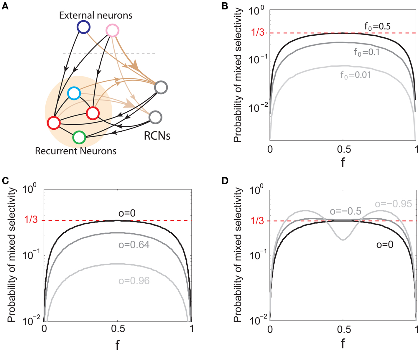
Figure 3. (A) Neural network architecture: randomly connected neurons (RCN) are connected both to the recurrent neurons and the external neurons by fixed random weights (brown). Each RCN projects back to the recurrent network by means of plastic synapses (black). Not all connections are shown. (B) Probability that an RCN displays mixed selectivity (on log scale) and hence solves the problem of Figure 2 as a function of f, the average fraction of input patterns to which each RCN responds. Different curves correspond to different coding levels f₀ of the representations of the mental states and the external inputs. The peak is always at f = 1/2 (dense RCN representations). (C) Probability that an RCN has mixed selectivity as a function of f, as in (B), for different positive values of the overlap o between the two initial mental states, and the two external inputs corresponding to the spontaneous activity and the event. Again the peak is always at f = 1/2. The curve decays gently as o goes to 1. (D) As in (C), but for negative values of the overlap o, meaning that the patterns representing the mental states are anti-correlated. There are now two peaks, but notice that they remain close to f = 1/2 for all values of o.

If the activity threshold θ = 0, then every RCN responds on average to half of all possible input patterns (dense coding), as the total synaptic current is either positive or negative with equal probability. As the threshold θ increases, an RCN responds to a progressively decreasing fraction f of input patterns (sparse coding). For example, an RCN that by chance is strongly connected to both the Shape Rule recurrent neurons and to the Error Signal external neurons, will have the same mixed selectivity as the neuron represented in Figure 2B. Indeed, for a sufficiently high threshold θ, it would respond to the Error Signal only when Shape Rule neurons are active. It turns out that the probability that an RCN, as a mixed selectivity neuron, responds to an odd number of the possible combinations of the external input and the inner mental state can be as large as 1/3 when θ is small and f is close to 1/2 (see Figure 3B and Estimating the Number of Needed RCNs in Appendix). Surprisingly, this result implies that the number of RCNs needed to solve a context-dependent problem is on average only three times larger than the number of neurons needed in a carefully designed neural circuit.

In general, the probability that an RCN is a mixed selectivity neuron, depends on the coding level f₀ (the fraction of active neurons in the recurrent and the external network), on the correlations between the representations of different mental states and different external inputs, and on the threshold θ that determines the coding level f of the RCNs. However, it does not depend on the values and the specific distribution of the random synaptic weights, provided that the synapses are not correlated to other synapses or to the input patterns. This means that the synaptic connections to the RCNs can be positive and negative, entirely positive (excitatory), or entirely negative (inhibitory), and the probability of finding a mixed selectivity neuron remains the same, provided that the threshold θ is properly shifted (see Estimating the Number of Needed RCNs in Appendix).

Dense representations of RCN patterns of activities (f = 1/2) are more efficient than sparse representations (f → 0 or f → 1), regardless of the coding level f₀ of the representations of the mental states and the external inputs. This is illustrated in Figure 3B where the probability that an RCN responds as a mixed selectivity neuron is plotted against f for three values of f₀. The proof is valid for patterns representing mental states and events that are random and uncorrelated. All curves have a maximum in correspondence of f = 1/2 and they are relatively flat for a wide range of f values. The maximum decreases gently as f₀ approaches 0 (approximately as ) because the overlap between different mental states and external inputs progressively increases, and this makes it difficult for an RCN to discriminate between different initial mental states, or different external inputs. For the same reasons, the maximum decreases in the same way as f₀ tends to 1.

As the patterns representing mental states and events become progressively more correlated, the number of needed RCNs increases. In particular, in Figure 3C we show the probability of mixed selectivity as a function of f of the RCNs for different correlation levels between the patterns representing mental states and external events. The degree of correlation is expressed as the average overlap o between the two patterns representing the initial mental states (the same overlap is used for the two external events). o varies between −1 and 1, and it is positive and close to 1 for highly similar patterns (Figure 3C) or negative (Figure 3D), for anti-correlated patterns. The overlap o = 0 corresponds to the case of uncorrelated patterns. As o increases, it becomes progressively more difficult to find an RCN that can have a differential response to the two initial mental states. This is reflected by a probability that decreases approximately as . For all curves plotted in Figure 3C, the maximum is always realized with f = 1/2. Interestingly, for anti-correlated patterns, the maximum splits in two maxima that are slightly above 1/3 (see Figure 3D). The maxima initially move away from f = 1/2 as the patterns become more anti-correlated, but then, for o < −5/6, they stop diverging from the mid point. The optimal value for f remains within the interval [0.3, 0.7] for the whole range of correlations.

In all the cases that we analyzed, which cover practically all possible statistics of the patterns for the mental states and the external events, the probability of finding an RCN that solves the context-dependent task is always surprisingly high, provided that the patterns of activities of the RCNs are not too sparse (i.e., when f is sufficiently close to 1/2, within the interval [0.3, 0.7]).

In this section we analyzed the probability that an RCN solves a single, generic, context-dependent problem. How does the number of needed RCNs scale with the complexity of an arbitrary task with multiple context dependencies? In order to answer this question, we first need to define the neural dynamics and construct a circuit that harnesses RCNs to implement an arbitrary scheme of mental states and event-driven transitions.

A General Recipe for Constructing Recurrent Networks that Implement Complex Tasks

Consider our model shown in Figure 3A. Given a scheme of mental states and event-driven transitions like the one of Figure 1B, the weights of the plastic synaptic connections are modified according to a prescription that guarantees that the mental states are stable patterns of activity (attractors) and that the events steer the activity toward the correct mental state. In particular, for each attractor encoding a mental state, and for each event-driven transition we modify the plastic synapses as illustrated in Figure 4. For the example of the transition Shape + Left to Color induced by an Error Signal of Figure 4A we clamp the recurrent neurons to the pattern of activity corresponding to the initial state (Shape + Left). We then compute the activity of the RCNs. We isolate in turn all the recurrent neurons and we modify their plastic synapses according to the perceptron learning rule (Rosenblatt, 1962) so that the total synaptic input drives the neurons to the activation state they should have at time t + Δt, after the transition has occurred. In case of the mental states we impose their stationarity by requiring that each pattern representing a mental state at time t reproduces itself at time t + Δt (see Figure 4B). In order to guarantee the stability of these patterns, we require that active neurons are driven by a current that is significantly larger than the minimal threshold value θ (i.e., I > θ + d, where d > 0 is known as a “learning margin”). Analogously, inactive neurons should be driven by a current I < θ − d. To avoid that the stability condition is trivially satisfied by inflating all synaptic weights, we require that the learning margin should grow with the length of the vector representing all the synaptic weights on the dendritic tree (Krauth and Mezard, 1987; Forrest, 1988) (see Methods: Details of the Model for the details of the synaptic dynamics). When the learning procedure is repeated for all neurons, the patterns of activity corresponding to the mental states are cooperatively maintained in time through synaptic interaction and are robust to perturbations.

FIGURE 4

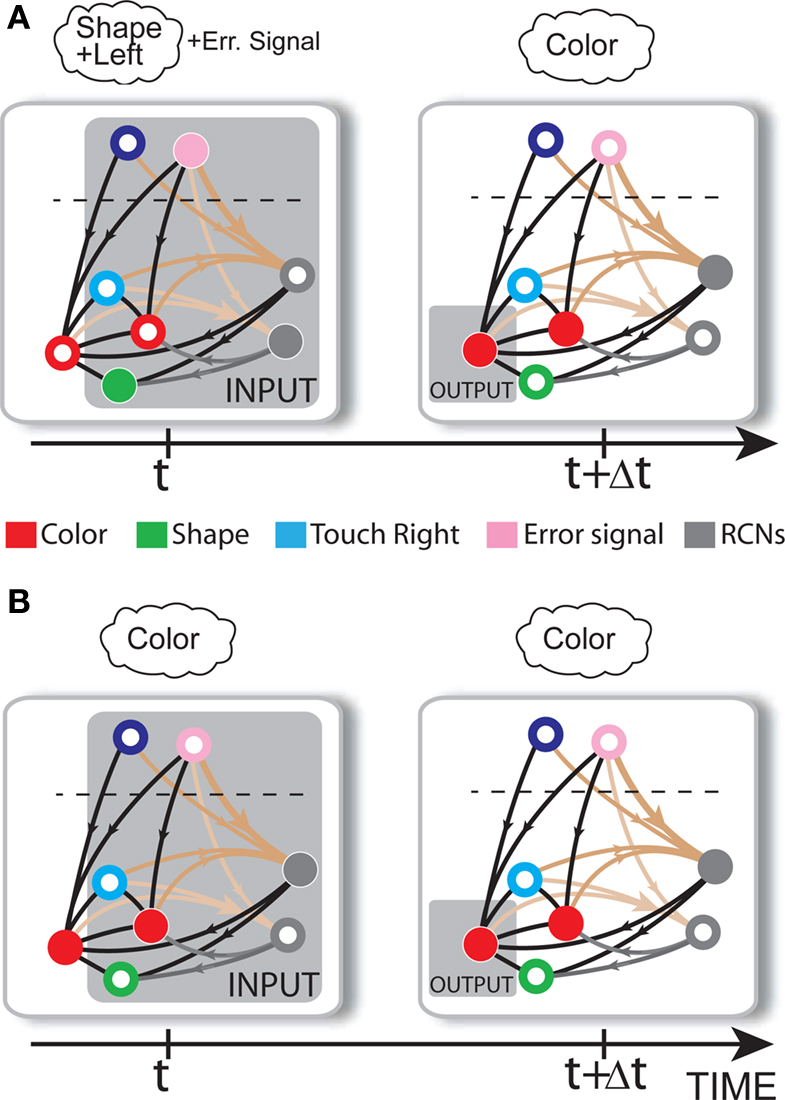
Figure 4. Prescription for determining the plastic synaptic weights. (A) For event-driven transitions the synapses are modified as illustrated in the case of the transition from Shape + Left to Color induced by an Error Signal. The pattern of activity corresponding to the initial attractor (Shape + Left) is imposed to the network. Each neuron is in turn isolated (leftmost red neuron in this example), and its afferent synapses are modified so that the total synaptic current generated by the initial pattern of activity (time t, denoted by INPUT), drives the neuron to the desired activity in the target attractor (OUTPUT at time t + Δt). (B) For the mental states the initial and the target patterns are the same. The figure shows the case of the stable pattern representing the Color mental state. The procedure is repeated for every neuron and every condition.

All conditions corresponding to the mental states and the event-driven transitions can be imposed if there is a sufficient number of RCNs in the network. If it is not possible to satisfy all conditions simultaneously we keep adding RCNs and we repeat the learning procedure. We show that such a procedure is guaranteed to converge (see Estimating the Number of Needed RCNs in Appendix).

Dense Neural Representations Require a Number of Neurons that Grows Only Linearly with the Number of Mental States

If we follow the prescription of the previous paragraph, how many RCNs do we need in order to implement a given scheme of mental states and event-driven transitions? Not surprisingly, the answer depends on the threshold θ for the activation of the RCNs, and hence on the RCNs’ coding level f. Indeed we have shown that the probability that an RCN solves a single context dependence problem depends on f, and that it is maximal for dense representations. We expected to observe a similar dependence in the full dynamic neural network implementing a complex scheme of multiple mental states and context-dependent event-driven transitions.

In the extreme limit of small f (ultra-sparse coding), each RCN responds only to a single, specific input pattern (f = 1/2^N, where 2^N is the total number of possible patterns and N is the number of synaptic inputs per RCN). We prove in Section “Estimating the Number of Needed RCNs” in Appendix that for the ultra-sparse case, any scheme of attractors and event-driven transitions can be implemented and the basins of attraction can have any arbitrary shape. Unfortunately, the number of necessary RCNs grows exponentially with the number of recurrent and external neurons. Such a dependence reflects the combinatorial explosion of possible patterns of neural activity that represent conjunctions of events.

On the other hand, with a larger f, it is more likely that an RCN solves our problem, as for the mixed selectivity neuron of Figure 2B. To quantify this effect we devised a benchmark to estimate how the number of necessary RCNs scales with f and the complexity of a context-dependent task in the case of multiple context dependencies. Specifically, we simulated a network with RCNs with coding level f implementing a set of r random transitions between m mental state attractors represented by random uncorrelated patterns. Since the result of a transition triggered by an external stimulus depends in general on the initial mental state, m can also be thought of as the number of distinct contexts. Additionally, in all these analyses we sought to make sure that the attractors representing the mental states had a finite basin of attraction ρ_B. This means that, whenever the activity pattern was in an initial configuration within a distance ρ_B > 0 from an attractor representing a mental state, then the network dynamics was required to relax into the corresponding attractor. Equivalently, every pattern of activity with an overlap greater than o = 1 − 2ρ_B with a given attractor pattern was required to evolve toward that attractor. For each set of parameters m, r, f, and ρ_B, we computed the minimal number of required total neurons in the network (recurrent and RCNs), so that the r transitions are correctly implemented and all the m mental states have a basin of attraction of at least ρ_B.

Figure 5A shows the required total number of neurons (recurrent and RCNs) as a function of the coding level f of the RCNs found by varying the number of neurons so that the RCNs were always four times as many as the recurrent neurons. The results are shown for r = m transitions for three different numbers of contexts, m = 5,10,20. Consistently with the estimates of the probability that an RCN solves a single context dependence problem plotted in Figure 3, the minimal number of required neurons is in correspondence of dense RCNs patterns of activity (f = 1/2). With f = 1/2, we examined in Figure 5B how the minimal number of needed neurons depends on the task complexity, and in particular how it depends on the number of mental states m and transitions r. Notice that for the curves in Figure 5B labeled with r > m, the same event drives more than one transition, which is what typically happens in context-dependent tasks. The total number of neurons needed to implement the scheme of mental states and event-driven transitions and to keep the size of the basins of attraction constant, increases linearly with m and the slope turns out to be approximately proportional to the ratio r/m, the number of contexts in which each event can appear. In other words, the number of needed neurons increases linearly with the total number of conditions to be imposed for the stability of mental states, and the event-driven transitions. This favorable scaling relation indicates that highly complicated schemes of attractor states and transitions can be implemented in a biological network with a relatively small number of neurons.

FIGURE 5

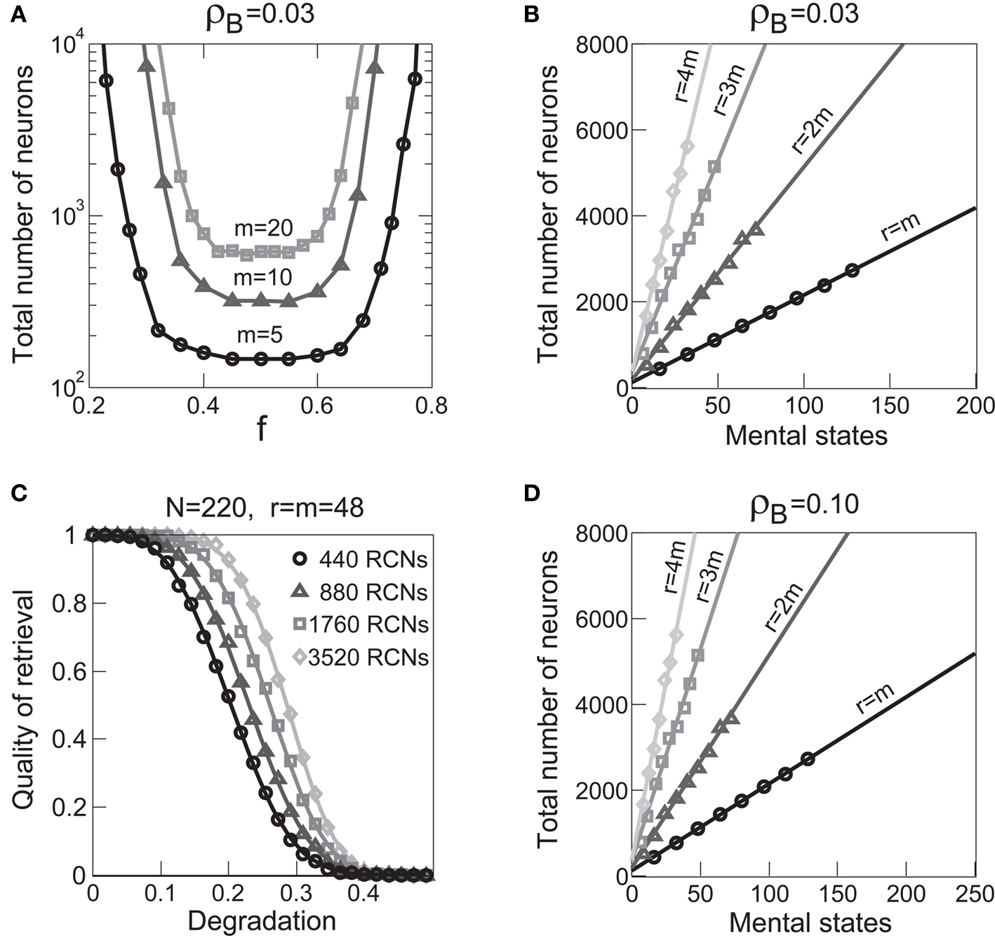
Figure 5. (A) Distributed/dense representations are the most efficient: total number of neurons (recurrent network neurons + RCNs) needed to implement r = m transitions between m random attractor states (internal mental states) as a function of f, the average fraction of inputs that activate each individual RCN. The minimal value is realized with f = 1/2. The three curves correspond to three different numbers of mental states m (5,10,20). The number of RCNs is 4/5 of the total number of neurons. (B) Total number of needed neurons to implement m random mental states and r transitions which are randomly chosen between mental states, with f = 1/2. The number of needed neurons grows linearly with m. Different curves correspond to different ratios between r and m. The size of the basin of attraction is at least ρ_B = 0.03 (i.e., all patterns with an overlap larger than o = 1 - 2ρ_B = 0.94 with the attractor are required to relax back into the attractor). (C) The size of basins of attraction increases with the number of RCNs. The quality of retrieval (fraction of cases in which the network dynamics flows to the correct attractor) is plotted against the distance between the initial pattern of activity and the attractor, that is the maximal level of degradation tolerated by the network to still be able to retrieve the attractor. The four curves correspond to four different numbers of RCNs. In all these simulations the number of recurrent neurons was kept fixed at N = 220 and m = r = 48. (D) Same as (B), but for larger basins of attraction, ρ_B = 0.10.

Scaling Properties of the Basins of Attraction

The RCNs have been introduced to solve the problems originated by the context dependence of some of the transitions. What is the effect of the RCNs on the size and the shape of the basins of attraction? The participation of the RCNs population in the network dynamics effectively leads to the dilation of the space in which the patterns of neural activity are embedded. Specifically, as the number of RCNs increases, the absolute distance between the activity vectors representing different combinations of mental states and external inputs also increases. As a result, the patterns of activity representing the mental state and the external input become more distinguishable and easily separable by read-out neurons. This projection into a higher dimensional space is remindful of the support vector machines (SVM) strategy of pre-processing the data (Cortes and Vapnik, 1995).

The space dilation caused by the introduction of the RCNs can solve the non-linear separabilities generated by context dependence. At the same time it has the desirable property of approximately preserving the structure of the basins of attraction. Indeed, the total synaptic inputs to the RCNs have statistical properties that are similar to the ones of random projections. Random projections are simply obtained by multiplying the vectors representing the patterns in the original space by a matrix with random uncorrelated components. These projections preserve vectors similarities with high probability if the projection space is large enough (Johnson and Lindenstrauss, 1984). As a consequence random projections preserve the structure of the basins of attraction, because all points surrounding the attractor in original space are mapped onto points which maintain the same spatial relation.

Because of the non-linearity due to the sigmoidal neuronal input–output relation, the RCNs distort the space and preserve similarities only with some degree of approximation. For instance, small distances are on average amplified more than large distances. However, similarly to what happens for random projections, the ranking of distances is preserved (again, on average). In other words, if pattern B is more similar to A than C, also the corresponding RCN representations will be likely to preserve the same similarity relations. This is an important property for preserving the topology of the basins of attraction.

To summarize, the RCNs always increase the absolute distances between the input patterns of activity and preserve approximately the relative distances. The small distortions introduced by the non-linear input–output function have the beneficial effect of solving the non-linear separability due to context dependence, and the negative effect of partially disrupting the topology of the basins of attraction.

The effect on the capacity are illustrated in Figures 5B–D. The basin of attraction for a fixed point is estimated in Figure 5C. Starting from the fixed point, we perturbed the neurons of the recurrent network, and measured the fraction of perturbed patterns that relaxed back into the correct attractor. The fraction of correct relaxations stays at 1 when the initial patterns are close to the attractor and then it decreases with the fraction of perturbed neurons. As long as the fraction of correct relaxations is near 1, most of the patterns are within the basin of attraction. The different curves correspond to a different number of RCNs (at fixed number of recurrent neurons) and it is clear that the introduction of RCNs expands the basin of attraction, although the number of required neurons seems to grow exponentially with the size of the basin.

However, when the complexity of the task increases, the dependence of the number of RCNs on the number of mental states and the number of transitions remains linear for all the different sizes of basins of attraction that we studied. In order to preserve this scaling, we increased in the same proportion the number of neurons of the recurrent network and the RCNs, so that the RCNs can solve the non-linear separabilities, but at the same time they do not distort too much the distances in the original space of the recurrent network. In Figure 5D we show how the number of required neurons (recurrent neurons + RCNs) scales with the number of mental states for the benchmark of Figure 5B. The two figures differ in the required sizes for the basins of attraction. For Figure 5B the basin of attraction had to be large enough to guarantee that initial patterns with a perturbation as high as 3% (i.e., the probability of changing the state of each neuron is ρ_B = 0.03) would all relax back in the attractor. In Figure 5D the requirement about the basin of attraction was that initial patterns with a 10% perturbation would all relax back in the attractor. In both cases the number of needed neurons is linear in both the number of mental states m and the number of transitions r. In particular, if N_r is the total number of required neurons, we have that:

N_r ∼ α(r/m)m,

where α is a function of the number of transitions per state (r/m). In our case, α = βr/m, where β depends on the size of the basins of attraction. It is practically constant for ρ_B = 0.03, 0.10 (β ≃ 60) and it increases rapidly for larger basins with ρ_B = 0.20 (β ≃ 200, not shown in the figures). Our simulations show in all cases that the number of needed neurons increases linearly with the number of conditions to be imposed (i.e., the number of attractors plus the number of event-driven transitions), regardless of the size of the basin of attraction.

The introduction of RCNs increases the absolute distances between the input patterns, and also has the beneficial effect of speeding up the learning process. Indeed the convergence time of the perceptron algorithm that we use to impose all the conditions for attractors and transitions decreases with an increasing number of RCNs, as shown in Section “The Number of Learning Epochs Decreases with the Number of RCNs” in Appendix, Figure 8. This is true also when we impose that the basins of attractions must have a given fixed size, or in other words, that the generalization ability of the network remains unchanged for different numbers of RCNs.

Modeling Rule-Based Behavior Observed in Monkey Experiments

The prescription for building neuronal circuits that implement a given scheme of mental states and event-driven transitions is general, and it can be used for arbitrary schemes provided that there is a sufficient number of RCNs. To test our general theory, we applied our approach to a biologically realistic neural network model designed to perform a rule-based task which is analog to the WCST described in Figure 1 (Mansouri et al., 2006, 2007), whose scheme is reproduced in Figure 7A. We implemented a network of more realistic rate-based model neurons with excitation mediated by AMPA and slow NMDA receptors, and inhibition mediated by GABA_A receptors. Figure 6A shows the simulated activities of two rule selective neurons during two consecutive trials after a rule shift. The rule in effect changes from Color to Shape just before the first trial, causing an erroneous response that is corrected in the second trial, after the switch to the alternative rule. Although the two neurons shown in Figure 6A are always selective to the rule, their activity is modulated by other events throughout all the epochs of the trials. This is due to the interaction with the other neurons in the recurrent network and with the RCNs. Figure 6B shows the activity of three RCNs. They typically have a rich behavior exhibiting mixed selectivity that changes depending on the epoch (and hence on the mental state). Two features of the simulated neurons have already been observed in experiments: (1) neurons show rule-selective activity in the inter-trial interval, as observed for a significant fraction of cells in PFC (Mansouri et al., 2006); (2) the selectivity to rules is intermittent, or in other words, neurons are selective to a different extent to the rules depending on the epoch of the trial. This second feature is analyzed in detail in the next section.

FIGURE 6

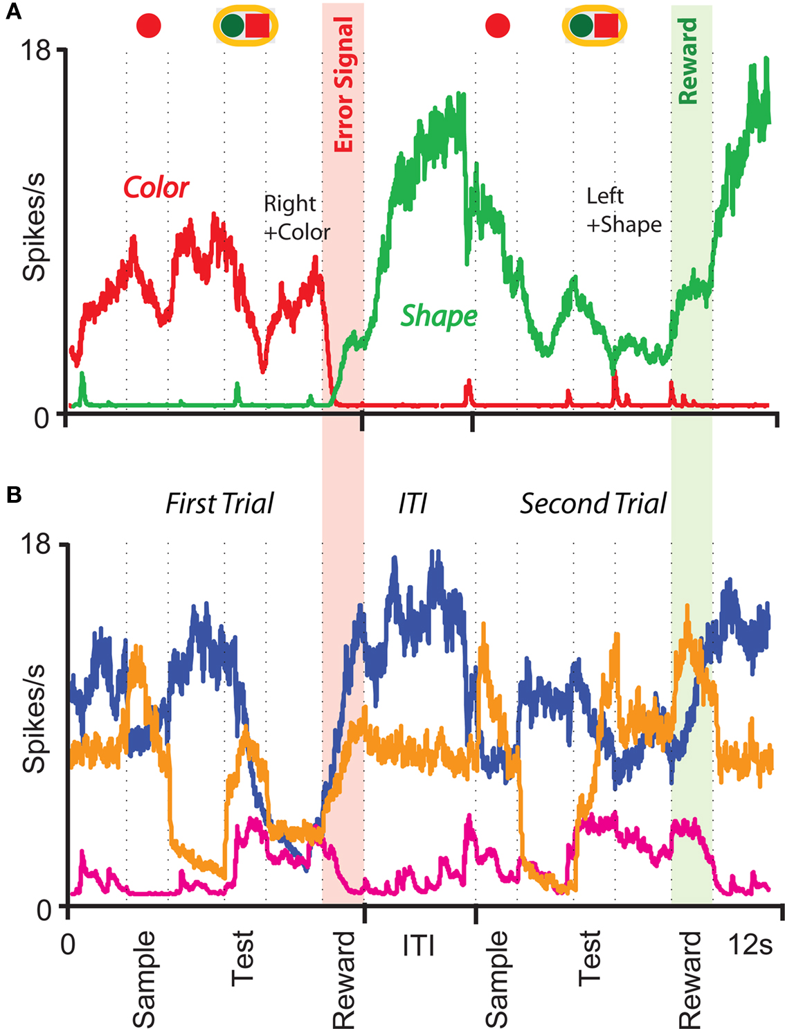
Figure 6. Simulation of a Wisconsin Card Sorting-type Task after a rule shift. (A) Simulated activity as a function of time of two sample neurons of the recurrent network that are rule selective. The first neuron (red) is selective to “color” and the second (green) to “shape”. The events and the mental states for some of the epochs of the two trials are reported above the traces. (B) Same as (A), but for three RCNs.

FIGURE 7

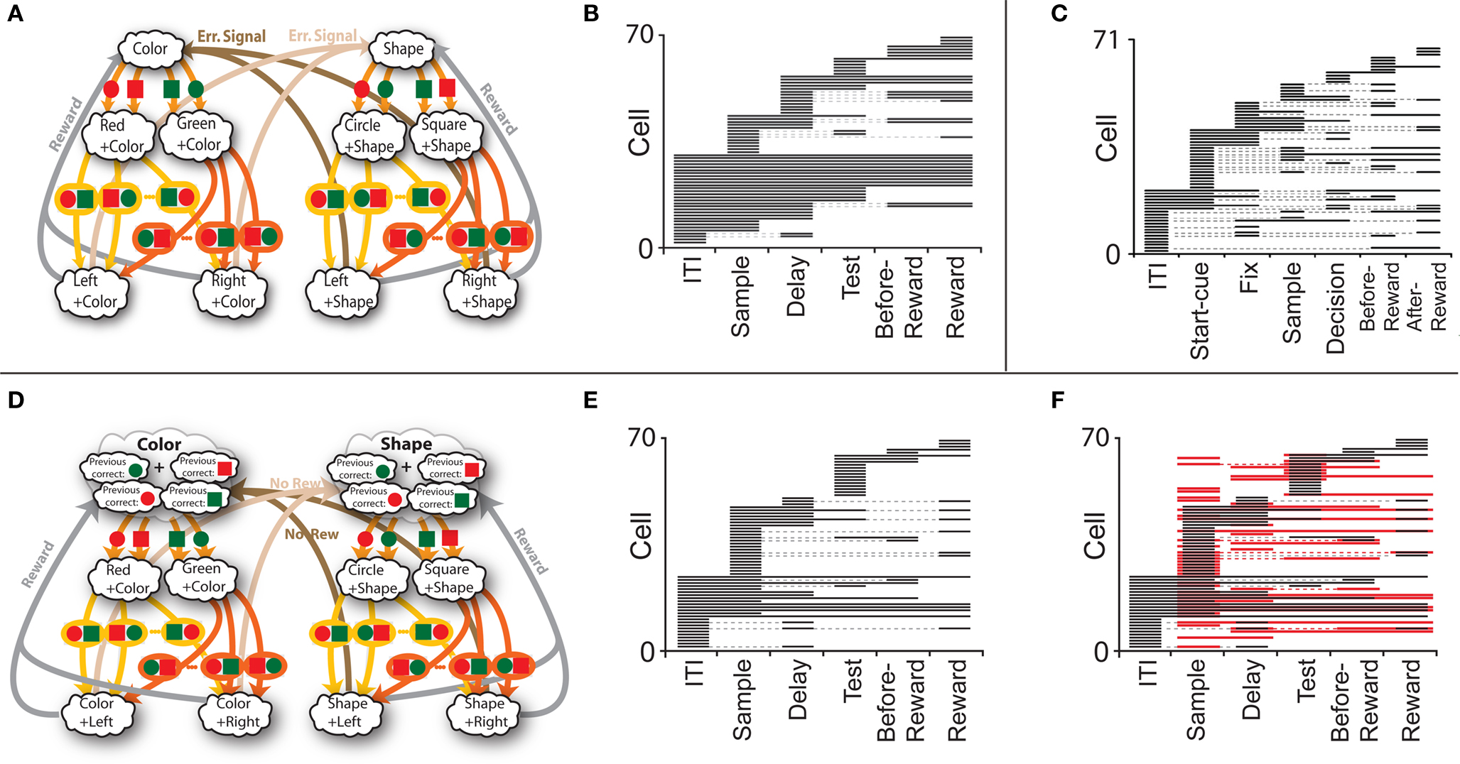
Figure 7. (A) Minimal scheme of mental states and event-driven transitions for the simplified WCST (same as in Figure 1B). (B) Rule selectivity pattern for 70 simulated cells: for every trial epoch (x-axis) we plotted a black bar when the neuron had a significantly different activity in shape and in color blocks. The neurons are sorted according to the first trial epoch in which they show rule selectivity. (C) Same analysis as in (B), but for spiking activity of single-units recorded in prefrontal cortex of monkeys performing an analog of the WCST (Mansouri et al., 2006). (D) Scheme of mental states and event-driven transitions with multiple states during the inter-trial interval (E) Same as (B), but for the history-dependent scheme in (D). (F) Same as (E), but for the selectivity to the color of the sample (red bars). Short black bars indicate rule selectivity.

Observed Properties of Mixed Selectivity Neurons: Intermittent Selectivity in Simulations and Experiments

To analyze more systematically the selectivity of simulated mixed selectivity cells and to compare it to what is observed in prefrontal cortex, in Figure 7B we plotted for 70 cells whether they are significantly selective to the rule for every epoch of the trial. The cells are sorted according to rule selectivity in different epochs, starting from the neurons that are rule selective in the inter-trial interval. Whenever a cell is rule selective in a particular epoch, we draw a black bar. In the absence of noise, all cells would be selective to the rule, as every mental state is characterized by a specific collective pattern of activity and the activity of each neuron is unlikely to be exactly the same for two different mental states. However we consider a cell to be selective to the rule only if there are significant differences between the average activity in Shape trials and the average activity in Color trials. The results depend on the amount of noise in the simulated network, but the general features of selectivity described below remain the same for a wide range of noise levels.

The selectivity clearly changes over time, as the set of accessible mental states for which the activity is significantly different, changes depending on the epoch of the trial. This intermittent selectivity is also observed in the experimental data (Mansouri et al., 2006) reproduced in Figure 7C. More recently it has been observed also in (Cromer et al., 2010). The experimental selectivity is in general less significant than in the simulations for several reasons. In the experiment the neural activity is estimated on a limited number of trials from spiking neurons and hence the noise can be significantly higher than in the simulations. However there might be a more profound reason for the discrepancy between experiments and simulations, which is related to the fact that the monkey might be using a strategy that is more complicated than the one represented in Figure 1B. If, indeed, we assume that the monkey keeps actively in mind not only the rule in effect, but also some other information about the previous trial that is not strictly essential for performing the task, then the number of accessible states during the inter-trial interval can be significantly larger, and this can strongly affect the selectivity pattern of Figure 7B. This is illustrated in Figures 7D–F, where we assumed that the monkey remembers not only the rule in effect, but also the last correct choice (see e.g., Barraclough et al., 2004 for a task in which the activity recorded in PFC contains information about reward history). In such a case the activity in the inter-trial interval is more variable from trial to trial and the pattern of selectivity resembles more closely the one observed in the experiment of Mansouri et al. (2006).

The statistics of the black bars depends on the structure of the neural representations of the mental states and on the statistics of the random connections to the RCNs. In particular, the correlations between mental states can generate correlations between patterns of selectivity in different epochs, and across neurons. The fact that rule selectivity is not a property inherent to the cell is a general feature of our network which will be demonstrated also for different types of selectivity, such as a stimulus feature or reward delivery (observed in the experiment of Mansouri et al., 2006). For example, the simulations in Figure 7F show for the same cells of Figure 7E the selectivity to the color of the sample stimulus (red bars), on top of the bars indicating rule selectivity. Obviously, there is no cell that is selective to the sample stimulus before it is presented (inter-trial interval), but in the remaining part of the trial the pattern of red bars seems to be as complex as the one for rule selectivity. Notice that some cells are selective to both the rule and the color in some epochs.

Predicted Features of Mixed Selectivity: Diversity, Pre-Existence, and Universality

The RCNs and the recurrent neurons show mixed selectivity that is predicted to exhibit features that are experimentally testable. In particular:

1. Mixed selectivity should be highly diverse, in time, as pointed out in the previous section (see also Lapish et al., 2008; Sigala et al., 2008), and in space, as different neurons exhibit significantly different patterns of selectivity. Such a diversity is predicted to be significantly higher than in the case of alternative models with hidden units, in which the synaptic connections are carefully chosen to have a minimal number of hidden units. According to our model, neurons with selectivity to behaviorally irrelevant conjunctions of events and mental states are predicted to be observable at any time (see Rigotti et al. (2010) for preliminary experimental evidence in orbito-frontal cortex and amygdala).

2. Mixed selectivity should pre-exist learning: neurons that are selective to behaviorally relevant conjunctions of mental states and events are predicted to be pre-existent to the learning procedure of a task.

3. Mixed selectivity should be “universal”: the neurons of the network have the necessary mixed selectivity to solve arbitrarily complicated tasks that involve the present and future mental states. Were we able to impose artificially an arbitrary pattern of activity representing a future mental state, we would observe neurons that are selective to conjunctions of that mental state and familiar or unfamiliar events, even before any learning takes place.

These three features are illustrated in Figure 8 where we make specific predictions in the case in which the simplified WCST illustrated in Figure 1 and analyzed in the previous section is modified to produce a rule switch whenever a tone is heard. We consider the situation in which the subject has already learned and is correctly performing the WCST. At some point, a new sensory stimulus (e.g., a tone) signals a rule switch, and the task is modified as indicated in Figure 8A. We now analyze the behavior of the simulated network before the new task is learned. Figures 8B,C show the activity of a few neurons as a function of time. The tone is a new event, and it is initially ignored by the network collective dynamics and the behavior is still controlled by the old scheme of mental states and event-driven transitions. In other words, the tone is unable to induce any transition from one mental state to another. In general the behavior would be unaffected by any distractor that is sufficiently dissimilar from the relevant sensory stimuli. This resistance to distractors has been observed in prefrontal circuits (Sakai et al., 2002).

FIGURE 8

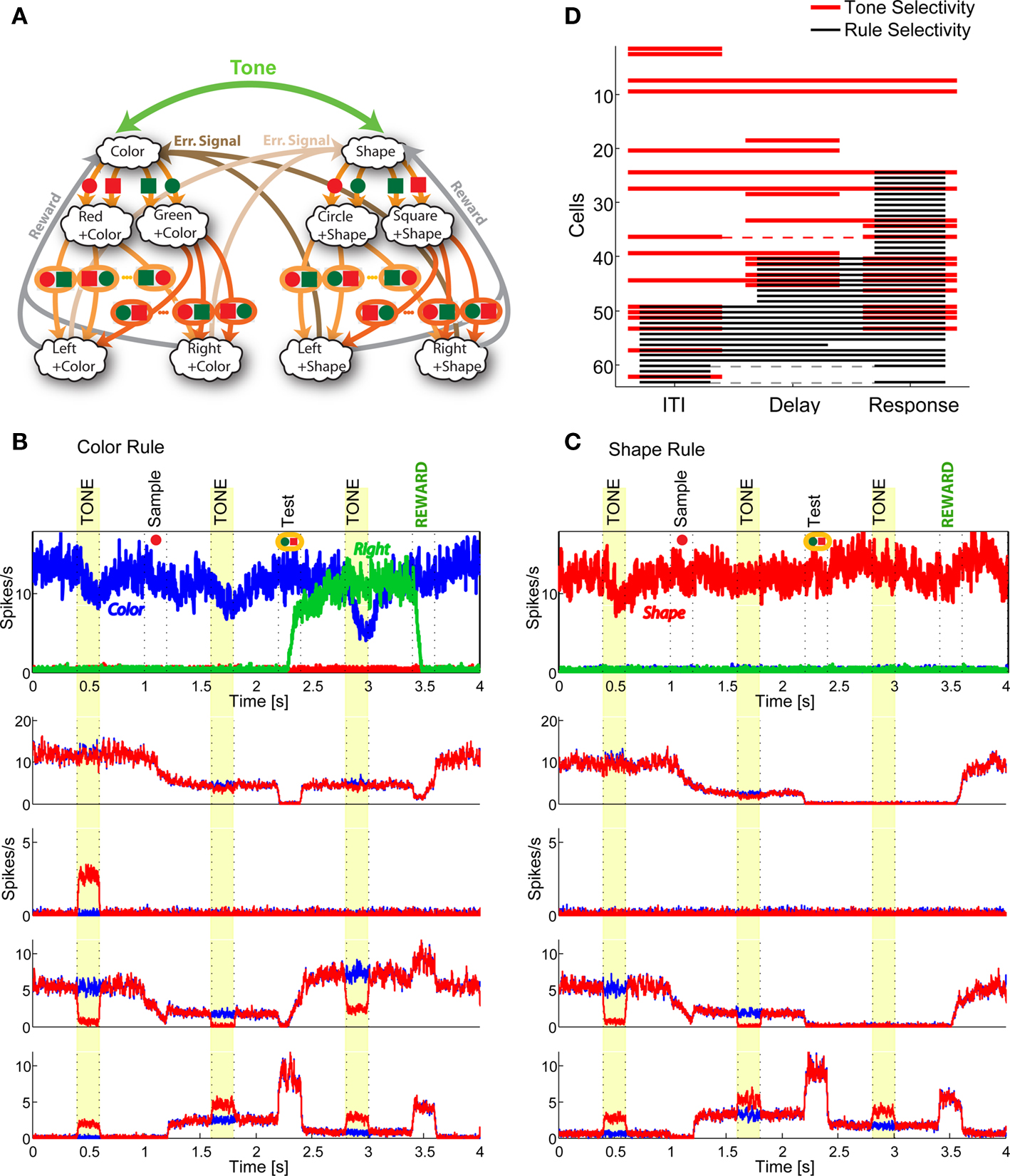
Figure 8. Diversity, pre-existence and universality of neurons with mixed selectivity. (A) Extended WCST (eWCST): task switch is driven not only by an error signal, but also by a tone (green arrow). (B,C) All necessary mixed selectivities are pre-existent (i.e., they exist before learning). The simulated network is trained on the WCST of Figure 1D. We show the neural activity in trials preceding learning of eWCST. The neurons in the top panels of (B,C) encode the rule in effect and the motor response Right, as in Figure 6. (B) Shows one trial in which Color Rule is in effect, (C) a trial in which Shape Rule is in effect. The other plots represent the activity of four cells during the same trial in the absence (blue) and in the presence (red) of the tone. Some neurons are selective to the rule, but not to the tone (top). Some others have mixed selectivity to the tone and the rule (two central panels) even when the conjunctions of events are still irrelevant for the task (the network is not trained to solve eWCST). See in particular the neuron in the top central panel, that responds to the tone only when Color Rule is in effect. Finally, there are neurons that are selective to the tone but not to the rule. (D) Selectivity to the rule in effect (black) and to the tone (red) before learning of the eWCST (cf. Figure 7F). There are many neurons with the mixed selectivity that are necessary to solve the eWCST before any learning takes place.

Although the tone does not initially induce any transition from one mental state to another, the activity of individual neurons is visibly affected by it, and there are clearly cells that are already selective to the conjunction of tone and mental states even before the meaning of the tone is learned. The selectivity to the tone is shown in the four bottom panels of Figures 8B,C, in which we plot the activity of a few representative RCNs in the presence (red) and in the absence of the tone (blue). These neurons clearly show a selectivity to the conjunction of tone and mental states (see yellow stripes).

This kind of behavior reflects an efficient form of gating that allows the neural network to perform correctly the task, but, at the same time, to encode transiently in its activity the occurrence of a new event (the tone).

It important to notice that these neurons that respond to conjunctions of tone and rule encoding mental states are irrelevant for the simplified WCST, but they are anyway present in the network and observable (high diversity feature). As it turns out, they are essential for rule switching induced by the tone, as they solve the context dependence problem of the task to be learned, and they are already present before the learning process takes place (pre-existence feature). The mixed selectivity of the RCNs is also universal, as it would solve any other task with elevated probability (universality feature). The statistics of the selectivity to rules and to the tone of 62 RCNs is shown in Figure 8D. The black bars represent selectivity to rules, as in Figures 7B,C,E, and the red ones represent selectivity to the tone. In both cases, the selectivity in the different epochs is shown before the learning process takes place. Figure 8D shows that there is a large proportion of RCNs that exhibit mixed selectivity to rules and tone, and that can greatly facilitate the learning process (see discussion in Asaad et al., 1998 and Rigotti et al., 2010).

Discussion

Heterogeneity is a salient yet puzzling characteristic of neural activity correlated with high level cognitive processes such as decision making, working memory, and flexible sensorimotor mapping. Usually models are built to reflect the way we believe the brain solves a certain problem, and neurons with particular functional properties are carefully chosen to make the system work. In some cases these systems are tested to see whether they remain robust in spite of the presence of disorder and the diversity observed in the real brain. Instead, here we showed that heterogeneity actually plays a fundamental computational role in complex, context-dependent tasks. Indeed, it is sufficient to introduce neurons that are randomly connected in order to reflect a mixture of neural activity encoding the internal mental state and the neural signals representing external events. The introduction of these cells in the network is sufficient to enable the network to perform complex cognitive tasks and facilitates the process of learning. One of the main results of our work is that the number of necessary randomly connected neurons is surprisingly small and typically is comparable to the number of cells needed in carefully designed neural circuits. The randomly connected neurons have the advantage that they provide the network with a large variety of mixed selectivity neurons from the very beginning, even before the animal can correctly perform the task. Moreover, when the representations are dense, they are “universal” as they are likely to participate in the dynamics of multiple tasks.

Other Approaches Based on Hidden Units with Mixed Selectivity

Mixed selectivity has already been proposed as a solution to similar and different problems. For example, mixed selectivity to the retinal location of a visual stimulus and the position of the eyes can be used to generate a representation of the position of external objects and then determine the changes in joint coordinates needed to reach the object (Zipser and Andersen, 1988; Pouget and Sejnowski, 1997; Pouget and Snyder, 2000; Salinas and Abbott, 2001). Neurons with these response properties have been observed in the parietal cortex of behaving monkeys. Neurons with mixed selectivity to the identity of a visual stimulus and its ordinal position in a sequence have been used to model serial working memory (Botvinick and Watanabe, 2007). Mixed selectivity to stimulus identity and to a context signal have been used to model visuomotor remapping (Salinas, 2004a). More in general, complex non-linear functions of the sensory inputs like motor commands, can be expressed as a linear combination of basis functions (Poggio, 1990). These non-linear functions can be implemented by summing the inputs generated by neurons with mixed selectivity to all possible combinations of the relevant aspects of the task (e.g., different features of the sensory stimuli). One of the unresolved issues related to this approach is that the number of needed mixed selectivity neurons increases exponentially with the number of relevant aspects of the task (combinatorial explosion). This should be contrasted with the linear scaling of our approach based on RCNs.

The solution that we propose is based on the introduction of additional neurons that are randomly connected and that modify the representation of inner mental states in the presence of external inputs. As discussed, our solution is simple and it reproduces the response properties of neurons recorded in prefrontal cortex. A similar solution to the context dependence problem has been proposed by Salinas (2004a,b), who harnessed gain modulation to solve the non-linear separabilities. His approach is similar to the basis function approach that was just discussed, in Section “Introduction,” as he introduces neurons whose activity depends on the product of a function of the identity of the stimulus and a function of the context signal. These neurons have mixed selectivity to the inner mental state encoding the context and to the sensory stimulus. Similarly to what we did with the RCNs, he also chose a random permutation of gain functions to generate these neurons. However, in contrast with what we did, the author decided not to model explicitly the neural circuit that maintains actively the context representation and produces the neurons with mixed selectivity. Moreover, and most importantly, he presented an interesting case study, but he did not study systematically the scaling properties of his neural system.

In the works discussed above, the neurons with mixed selectivity are the result of specific, prescribed synaptic weights. However, there are also more general learning rules to find the weights to hidden units that have the needed mixed selectivity. A classical example is the Boltzmann machine (Ackley et al., 1985), which has been designed to solve similar problems, in which attractors corresponding to non-linearly separable patterns are stabilized by the activity of hidden units. Recent extensions of the Boltzmann machine algorithm (O’Reilly and Munakata, 2000; Hinton and Salakhutdinov, 2006) can also deal with event-driven transitions from one attractor to another. Our approach is similar because our RCNs are analogous to the hidden units of the Boltzmann machines. However, in our case the synaptic connections to the RCNs are not plastic and we do not need to learn them.

We would like to stress that what we propose is not a real learning algorithm, but rather a prescription for finding the synaptic weights. A real, biologically plausible learning algorithm would probably require a significantly more complicated system, with many of the features discussed in O’Reilly and Munakata (2000). However we believe that it is important to notice that our network can implement arbitrarily complicated schemes of attractors and event-driven transitions with a very simple prescription to find the desired synaptic configuration. This might greatly simplify and speed up a real learning algorithm. Moreover, mixed selectivity neurons that are predicted to be present even before the learning procedure starts, can be used to learn mental states that represent rules or other abstract concepts. One example is the creation of mental states corresponding to different temporal contexts as considered in Rigotti et al. (2010). Recently, it has also been shown (Dayan, 2007) that mixed selectivity neurons implemented with multilinear functions can play an important role in neural systems that implement both habits and rules during the process of learning of complex cognitive tasks. Multilinearity implements conditional maps between the sensory input, the working memory state, and an output representing the motor response.

We assumed that the RCNs have fixed random synapses, but this does not imply that our network requires the existence of synapses that are not plastic. It might be possible that the statistics of the random synaptic weights varies on a timescale that is significantly longer than the timescales over which the tasks are learned. We still do not know whether the introduction of this form of learning can improve the performance of the network and to what extent, although we know that in general learning on multiple timescales can be greatly beneficial for memory performance (Fusi et al., 2005). We know that there are forms of learning rules that modify the synaptic weights of neurons that are initially randomly connected without disrupting the performance of the network. This is the case of multilayer perceptrons with synapses that are initialized at random values, as discussed below.

Other Models Based on Randomly Connected Neurons

Networks of randomly connected neurons have been studied since the 1960s (Marr, 1969; Albus, 1971). In these works the authors, inspired by the ideas by P. H. Greene (Greene, 1965), realized that random subsets of input patterns can provide an efficient, compact representation of the information contained in the patterns. At the same time, these representations can be less correlated than the original patterns, and hence they can facilitate learning and memorization. In the neural circuit that we propose, we basically create with the RCNs a compressed representation of the inner mental state and the external input, and in this sense the RCNs play a similar role to the neurons of Greene (1965), Marr (1969), and Albus (1971). Moreover, the non-linearity introduced by the f–I curve of the RCNs contributes to increase the distances between highly correlated patterns, similarly to the non-linearities introduced in the cited works. It is important to notice that the RCNs provide our recurrent circuit with an explicit dynamical process that decorrelates the patterns representing the mental states and the external inputs and, at the same time, it the distances are dilated without disrupting the structure of the basins of attraction (see Scaling Properties of the Basins of Attraction). Simplified models in which the patterns of activity are assumed to be random and uncorrelated do not explicitly address the issue of how the original representations are decorrelated, and whether the topology of the basins of attraction is preserved (see e.g., Hopfield, 1982 for a classic example and Cerasti and Treves, 2010 for a more recent application of the same idea to the feed-forward pre-processing performed by the dentate-gyrus).

More recently randomly connected neurons have been used to generate complex temporal sequences and time varying input–output relations (Maass et al., 2002; Jaeger and Haas, 2004; Sussillo and Abbott, 2009) and to compress, transmit and decompress information (Candes and Tao, 2004). In many other cases they also have been used implicitly in the form of random initial weights. For example in the case of gradient descent learning algorithms like backpropagation (Zipser and Andersen, 1988). As proved in our manuscript, much of the needed mixed selectivity to solve non-linear separabilities might be already present in the initial conditions when the synaptic weights of hidden units start from a random configuration. We suspect that in many situations the learning rules would not need to modify these synapses to achieve a similar performance.

How Dense Should Neural Representations be?

Our results show that in order to solve the problems related to context dependence, the optimal representations for mental states, external inputs and for the patterns of activities of the RCNs should be dense. This means that the majority of the neurons is expected to respond to a large fraction of aspects of the task, and in general to complex conjunctions of events and inner mental states. Despite the lack of systematic studies providing a direct quantitative estimate of the average coding level f, dense representations have been widely reported in prefrontal cortex (Fuster and Alexander, 1971; Funahashi et al., 1989; Miller et al., 1996; Romo et al., 1999; Wallis et al., 2001; Nieder and Miller, 2003; Genovesio et al., 2005; Mansouri et al., 2006, 2007; Tanji and Hoshi, 2008).

The optimal fraction f for solving context dependence problems is 1/2, and this is not surprising as such a fraction would maximize the amount of information that can be stored in the neural patterns of activity of the RCNs. Indeed RCNs have to provide the network with patterns of activities that contain the information about both the inner mental states and the external inputs. However, the observed f might be smaller than the optimal value 1/2 for at least two reasons. The first one is related to metabolic costs, as it is clear that sparser representations (small f) would require a lower neural activity and hence a lower energy consumption. The second one concerns the interference between different mental states. The same network has probably to solve also non-context-dependent tasks or subtasks, like simple one-to-one mappings. In such a case, elevated values of f can degrade the performance because of the interference of the memorized representations of the mental states, as already shown by several works on the importance of sparseness for attractor neural networks (see e.g., Amit, 1989). Fortunately, Figure 3B show that the probability that an RCN solves a context-dependent problem is nearly flat around the maximum at f = 1/2, and it decreases rapidly only for significantly sparse representations. The optimal f when all these factors are considered, is more likely to be in an interval like 0.1 − 0.5.

Stochastic Transitions

In our simulations of a WCST-type task, a transition from one rule to another was induced deterministically by an Error Signal or by the absence of an expected reward. However the parameters of the network and the synaptic couplings can be tuned in such a way that certain transitions between states occur stochastically with some probability (see Stochastic Transitions Between Mental States in Appendix). Such a probability might depend on the production of neuromodulators like acetylcholine or norepinephrine, which have been hypothesized to signal expected and unexpected uncertainty (Yu and Dayan, 2005). In uncertain environments, where reward is not obtained with certainty even when the task is performed correctly, the animal should accumulate enough evidence before switching to a different strategy. Such a behavior could be implemented by assuming that an independent system keeps track of recent reward history and produces a neuromodulator controlling the probability of making a transition between the mental states corresponding to alternative strategies. This scenario could explain the observed behavior of the monkeys in the WCST-type task (Mansouri et al., 2006, 2007) in which, when task rule switching was signaled by change of reward contingencies, they switched to a different rule with a probability close to 50%. A detailed analysis of the monkey behavior in the particular experiment that we modeled would be very interesting but goes beyond the scope of this work.

Why Attractors?

One of the limitations on the number of implementable transitions in the absence of mixed selectivity units is due to the constraints related to the assumption that initial states are stable patterns of persistent activity, or, in other words, attractors of the neural dynamics. This is based on the assumption that rules are encoded and maintained internally over time as persistent neural activity patterns (Goldman-Rakic, 1987; Amit, 1989; Miller and Cohen, 2001; Wang, 2001). Given the price we have to pay, what is the computational advantage of representing mental states with attractors? One of the greatest advantages resides in the ability to generalize to different event timings, for instance to maintain internally a task rule as long as demanded behaviorally. In most tasks, all animals have a remarkable ability to disregard the information about the exact timing when such an information is irrelevant. For example when they have to remember only the sequence of events, and not the time at which they occur. The proposed attractor neural networks with event-driven transitions can generalize to any timing without the necessity of re-training. Generalizing to different timings is a problem for alternative approaches that encode all the detailed time information (Maass et al., 2002, 2007; Jaeger and Haas, 2004) or for feed-forward models of working memory (Goldman, 2009). The networks proposed in Maass et al. (2002), Jaeger and Haas (2004), and Goldman (2009) can passively remember a series of past events, in the best case as in a delay line (Ganguli et al., 2008). The use of an abstract rule to solve a task requires more than a delay line for at least two reasons: (1) Delay lines can be used to generate an input that encodes the past sequence of recent events and such an input can in principle be used to train a network to respond correctly in multiple contexts. However, the combinatorial explosion of all possible temporal sequences would make training costly and inefficient as the network should be able to recognize the sequences corresponding to all possible instantiations of the rules. (2) Even if it is possible to train the network on all possible instantiations of the rule, it is still extremely difficult if not impossible to train the network on all possible timings. A delay line would consider distinct two temporal sequences of events in which the event timings are different, whereas any attractor based solution would immediately generalize to any timing.

Models of working memory based on short term synaptic plasticity (Hempel et al., 2000; Mongillo et al., 2008) can operate in a regime that is also insensitive to timing, but they require the presence of persistent activity and the imposition of the stability conditions on the synaptic matrix, similarly to what we proposed in our approach. Moreover, these attractor networks do not act like fast switches between steady states, instead they are endowed with slow recurrent dynamics and exhibit transients such as quasi-linear ramping activity on the timescale of up to a second (Wang, 2008, 2002).

Conclusion

Mixed selectivity allows the network to encode a large number of facts, memories, events, intentions and, most importantly, various combinations of them without the need of an unrealistically large number of neurons when the representations are dense. The necessary mixed selectivity can be easily obtained by introducing neurons that are connected randomly to other neurons, and they do not require any training procedure. The present work suggests that the commonly observed mixed selectivity of neural activity in the prefrontal cortex is important to enable this cortical area to subserve flexible cognitive behavior.

Methods: Details of the Model

To examine the scaling behavior of our network in the limit of a large number of neurons, we used a network of simplified firing-rate model neurons. This model was used to generate Figures 5 and A7. We then implemented a more complex, realistic, rate-based neural network model to simulate a version of the Wisconsin Card Sorting Test (Figures 6A,B, 7B,E,F, 8, and A9).

The Simplified Firing-Rate Network

Network architecture

The architecture of the neural network is illustrated in Figure 3A. There are three populations of cells: (1) the recurrent neurons, whose patterns of activity encode the inner mental state, (2) the external neurons, encoding the events that drive the transitions from one mental state to another, and representing the input neurons that are presumably in different brain areas and (3) the Randomly Connected Neurons (RCN), that provide the network with mixed selectivity neurons. The recurrent neurons receive input from themselves and the other two populations and project back to themselves and the RCNs. The RCNs receive input from both the external neurons and the recurrent network, and project back to the recurrent neurons, but, for simplicity, they are not connected among themselves. The external neurons do not receive any feedback from the other two populations.

All connections to the neurons in the recurrent network are plastic, whereas the connections to the RCNs are fixed, random and uncorrelated. The random connections to an RCN are Gauss distributed with zero mean and with a variance equal to 1/N, where N is the number of pre-synaptic neurons.

Neural dynamics

The recurrent neurons are simplified McCulloch–Pitts-like neurons whose activity is described by a continuous valued variable which varies between −1 and 1. Their dynamics is governed by the equation:

where τ = 5 ms, φ(x) = tanh(x), θ_i is a threshold, and I_i is the total synaptic current generated by all the afferent neurons (recurrent, RCNs and external):

Here J^r is the matrix of the plastic recurrent connections, J^rcn are the plastic connections from the RCNs to the recurrent network, and J^x is the matrix of the plastic synaptic connections from the external neurons to the recurrent neurons. Notice that for these simplified neurons both the neural activity ν_i and the synaptic connections can be positive or negative. The activity of the RCNs and of the external neurons are denoted by , respectively. The dynamics of the RCNs is governed by the same differential equation as the recurrent neurons, with the only difference that the total synaptic current is given by , where K^r and K^x are the afferent random connections from the recurrent network and from the external neurons, respectively. The integration time τ plays a role analogous to the transmission delays used in Sompolinsky and Kanter (1986) to implement transitions in temporal sequences of patterns of neural activities.

In the absence of any stimulus, the values are set to a fixed pattern of neural activities chosen at random with the same statistics of the patterns representing an external event. We will name “spontaneous” activity pattern. When an external event occurs, the values are set to the pattern representing the event for a duration of 2τ, and then are set back to .

The Prescription for Determining the Synaptic Weights

The plastic connections J^r, J^rcn and J^x are determined by imposing the mathematical conditions that ensure both the stability of the patterns of activity representing the mental states and the correct implementation of the event-driven transitions.

The first step is to analyze the task to be performed and construct a scheme of mental states and event-driven transitions like the one of Figure 1B. Notice that in general there are multiple schemes corresponding to different strategies for performing the same task. The second step is to choose the patterns of neural activities representing the mental states (for recurrent neurons) and the external events (for the external neurons). The structure of these patterns is normally the result of a complex procedure of learning whose analysis is beyond the scope of this work. However the prescription for constructing the neural network applies to any neural representation. The patterns we chose were all vectors with components ν_i = ±1.

The third step is to go iteratively over all mental state attractors and event drive transitions and modify the weights of the plastic synaptic connections until all mathematical conditions for the stability of the attractors and the event-driven transitions are satisfied. The algorithm is illustrated in Figures 4A,B where we show two snapshots of neural activity that are contiguous in time. For each transition from one initial attractor to a target attractor we set the external input to the pattern of activity that corresponds to the triggering event (see Figure 4A). At the same time we impose the pattern of activity of the initial attractor on the recurrent network. We then compute the activity of the RCNs at fixed external and recurrent neuronal activity. For each neuron in the recurrent network we compute the total synaptic current generated by the activity imposed on the other neurons and we modify the synapses in such a way that the current drives the neuron to the state of activation at time t + Δt. In particular the synaptic currents at time t will generate an activity pattern, under the assumption that the post-synaptic neurons will fire if and only if the total input currents are above the firing threshold θ. The synaptic weights are updated only if the synaptic currents do not match the output activities in the target attractor (i.e., the pattern of activity at time t + Δt), as in the perceptron learning algorithm (Rosenblatt, 1962). If they need to be modified, the synaptic weights are increased by a quantity proportional to the product of the pre-synaptic activity at time t and the desired post-synaptic activity (i.e., the pattern of active and inactive neurons at time t + Δt in the figure). The stationarity of the patterns of activity corresponding to the mental states is imposed in a similar way, by requiring that the pattern at time t generates itself at time t + Δt (see Figure 4B). Such a procedure is iterated until all conditions are simultaneously satisfied, guaranteeing that the patterns of activity of the desired attractors are fixed points of the neural dynamics and that the transitions are implemented in a one-step dynamics.

In order to have attractors, the fixed points should also be stable. This can be achieved by requiring that the total synaptic currents not only satisfy the desired conditions, but also that they are far enough from the threshold θ (Krauth and Mezard, 1987; Forrest, 1988). In this way, small perturbations of the input modify the total synaptic current, but not the state of activation of the neurons. The distance from the threshold is usually named learning margin, which we will denote by d. The synapses are updated until

ν_i(t + Δt)(I_i(t) − θ_i) > d > 0,

where I_i(t) is the total synaptic current to neuron i, θ_i is its firing threshold, and ν_i(t + Δt) is the desired output activity. In other words, synapses are updated as long as I_i(t) does not surpass θ_i + d when neuron i is required to be active at time t + Δt. Analogously, the synapses are modified until I_i(t) goes below θ_i − d when the desired output is inactive (ν_i(t + Δt) = −1).

These conditions can be easily satisfied by scaling up all synaptic weights by the same factor. For example, consider the case in which ν_i(I_i − θ_i) = d′ < d. If all synapses are multiplied by a factor a, then I_i → aI_i, and there is always an a such that the condition ν_i(aI_i − θ_i) > d is satisfied. This implies that it is possible to satisfy the condition also in situations when stability is not guaranteed. To avoid this problem we block synaptic updates only when (Krauth and Mezard, 1987; Forrest, 1988)

where γ is the stability parameter, and the J_ijs are the synapses that are afferent to neurons i. The stability parameter γ is chosen to be maximal, i.e., we progressively increase γ until the algorithm stops converging within a reasonable number of learning epochs (we chose 500). Such a procedure is similar to one of the γ-margin modified perceptron algorithms presented in Korzen and Klesk (2008), and allows us to approximately maximize the size of the basin of attraction of the stable patterns of activities corresponding to the mental states (Forrest, 1988). Summarizing, the equation for updating a synaptic weight J_ij is:

where Θ is the Heaviside function and the learning rate λ is set to 0.01.

Definition of the Size ρ_B of the Basin of Attraction

An attractor has a basin of attraction of size at least ρ_B, if the network dynamics evolves toward the attractor whenever it starts from activity patterns within a distance ρ_B from the attractor. In the simplified firing-rate network, we verify whether an attractor has a size ρ_B with the following procedure. For each attractor , (i = 1,…,N) we set the initial activity of the recurrent network to a pattern which differs from by a fraction ρ_B of neurons: for ρ_BN randomly chosen indices i ( for the remaining (1 − ρ_B)N neurons). Flipping the pattern of activity of the recurrent network, also causes some RCNs to flip. Once the recurrent network is set to the perturbed pattern of activity ( for i = 1,…,N) and the RCN network is set to the corresponding pattern, we run the neural dynamics (Eq. 1) for a time T = 10τ. We then verify whether the recurrent network evolved toward the attractor by calculating the overlap o^μ(T) at time T between and the resulting activity of the recurrent network . The overlap is defined as . We count the initial pattern as being in the basin of attraction of if and only if this overlap is higher than 0.99. This procedure was typically repeated for 20–100 randomly chosen initial patterns , all at distance ρ_B from ξ^μ. If all resulted as being in the basin of attraction of ξ^μ, then we defined ξ^μ as having a basin of attraction of size at least ρ_B.

Biologically Realistic Firing-Rate Model

Figures 6A,B show simulations of a biologically more realistic firing-rate model, in which separate excitatory and inhibitory neurons are connected through NMDA, AMPA, and GABA mediated synaptic currents. We started by training the synaptic weights of a simplified neural network of McCulloch–Pitts neurons, as described in the previous section. For the simulations of Figure 6 we implemented the scheme of mental states and transitions of Figure 1B. For the neural representations of mental states and external inputs, we used N^r = 8 neurons for the recurrent network, 2 encoding the rule (color, shape), 4 for the identity of the sample stimulus (2 colors and 2 shapes), and 2 for the motor responses (touch left, or touch right). These representations result in highly correlated patterns of mental states. The external stimuli are represented by N^x = 14 neurons: four indicating the color and the shape of the Sample stimulus, eight representing the color and shape of the two Test stimuli, and two representing either the Reward or NoReward. We used 384 RCNs, that is slightly more than a 16-fold amount of the total number of recurrent and external neurons.

After convergence of the learning prescription for the chosen representations of states and scheme of transitions, we obtained a matrix J of synaptic weights, which in general can be both positive and negative. To enforce Dale’s law, we separated excitation and inhibition by introducing a population of inhibitory neurons whose activity is a linear function of the total synaptic input generated by the excitatory neurons. In practice we rewrote the synaptic matrix J as:

where J⁻ is the absolute value of the most negative synapse and the ’s are all positive. J⁻ can be interpreted as the product of the synaptic strengths from excitatory to inhibitory and from inhibitory to excitatory neurons when the transfer function for the inhibitory neurons is linear. We followed a similar procedure for the RCNs, by replacing each of them with an excitatory neuron, and introducing a second inhibitory population that allows the connections projecting from the neurons replacing the RCNs to be always positive.

The activity of the excitatory and inhibitory neurons are denoted by the firing rates and ν^I, respectively. The equations governing the dynamics of these firing rates are:

where F is a threshold linear function with unitary gain: F(x) = x if X > 0; 0 otherwise, the currents are generated by the neurons representing the external events, and the synaptic currents are generated by the population of neurons y and injected into population x (x,y = E,I where E and I indicate excitatory and inhibitory neurons respectively). The time development of the synaptic currents is governed by:

where J^xy is a matrix of synaptic weights. The synaptic currents from excitatory to excitatory neuron (xy = EE) are mediated by NMDA receptor channels with a slow timescale τ_EE = τ_NMDA = 100 ms. They saturate at high frequencies ν_js of the pre-synaptic spikes due to the saturation of the open channels with slow decay rate (Wang, 1999; Brunel and Wang, 2001):

Currents from excitatory to inhibitory neurons (xy = IE) are mediated by fast excitatory AMPA synapses with τ_IE = τ_AMPA = 5 ms and φ_IE(ν_i) = ν_i. Finally, for xy = II (inhibitory self-couplings) and xy = EI (inhibitory to excitatory) we have GABA synapses with τ_xy = τ_GABA = 2 ms and φ_xy(ν_i) = ν_i. The synaptic matrices J^IE, J^II, J^EI have been chosen so that the total inhibitory current to the excitatory population is proportional to , where J⁻ is the most negative synapse obtained by the learning procedure. This condition can be expressed as:

J⁻ = −J^EI(1 + |J^II|)⁻¹J^IE.

Given a set of excitatory synaptic weights J^EE, it is always possible to compute a J^II large enough so that all fixed points are stable. Then the product J^EIJ^IE is determined by the above expression for a given J⁻. We chose without any loss of generality J^EI = 1 and J^IE = −J⁻(1 + |J^II|).

The network is set to its initial conditions simply by clamping the firing rates of the recurrent and of the external neurons to the pattern of activity representing the desired starting attractor and the “spontaneous activity” stimulus pattern, respectively, and letting all the currents and firing rates variables of the other neurons evolve according to Eqs 4 and 3 until a stationary state is reached.

External events are simulated by changing the activities of the external neurons to the pattern representing the event for a time Δt = 2τ_NMDA, where τ_NMDA is the longest synaptic time scale, and then setting them back to the spontaneous activity pattern.

Additionally, we introduced a multiplicative noise term that modifies the firing rate of the excitatory neurons . This term is meant to capture finite-size fluctuations widely studied in networks of integrate-and-fire neurons (Brunel and Hakim, 1999). Formally this is expressed by the following change in Eq. 3:

where η(t) is a Gaussian process with unitary variance and σ² = 0.01.

Appendix

Constraints on the Types of Implementable Context-Dependent Transitions

A geometrical representation of the context dependence problem

We now go back to consider the rule-selective neuron i in the recurrent network of Section “Fundamental Difficulties in Context-Dependent Tasks”. The implementation of a context-dependent task can be interpreted as a classification of presynaptic inputs. The correlations between the inputs make the patterns classified by neuron i non-linearly separable, or equivalent to the computation of the XOR (exclusive OR) operator (Minsky and Papert, 1969). Neuron i is indeed required to perform a computation which is equivalent to an XOR of the input generated by the recurrent network and the external input: when the external input is inactive, neuron i has to be active in one mental state, inactive in the other, whereas the activated external input requires neuron i to switch to a different state of activation. Figure A1B shows a graphical representation of the problem in the specific case of the simplified WCST, and in particular when is the mental state Shape + Left, is Color + Left, and E is the Error Signal.

FIGURE A1

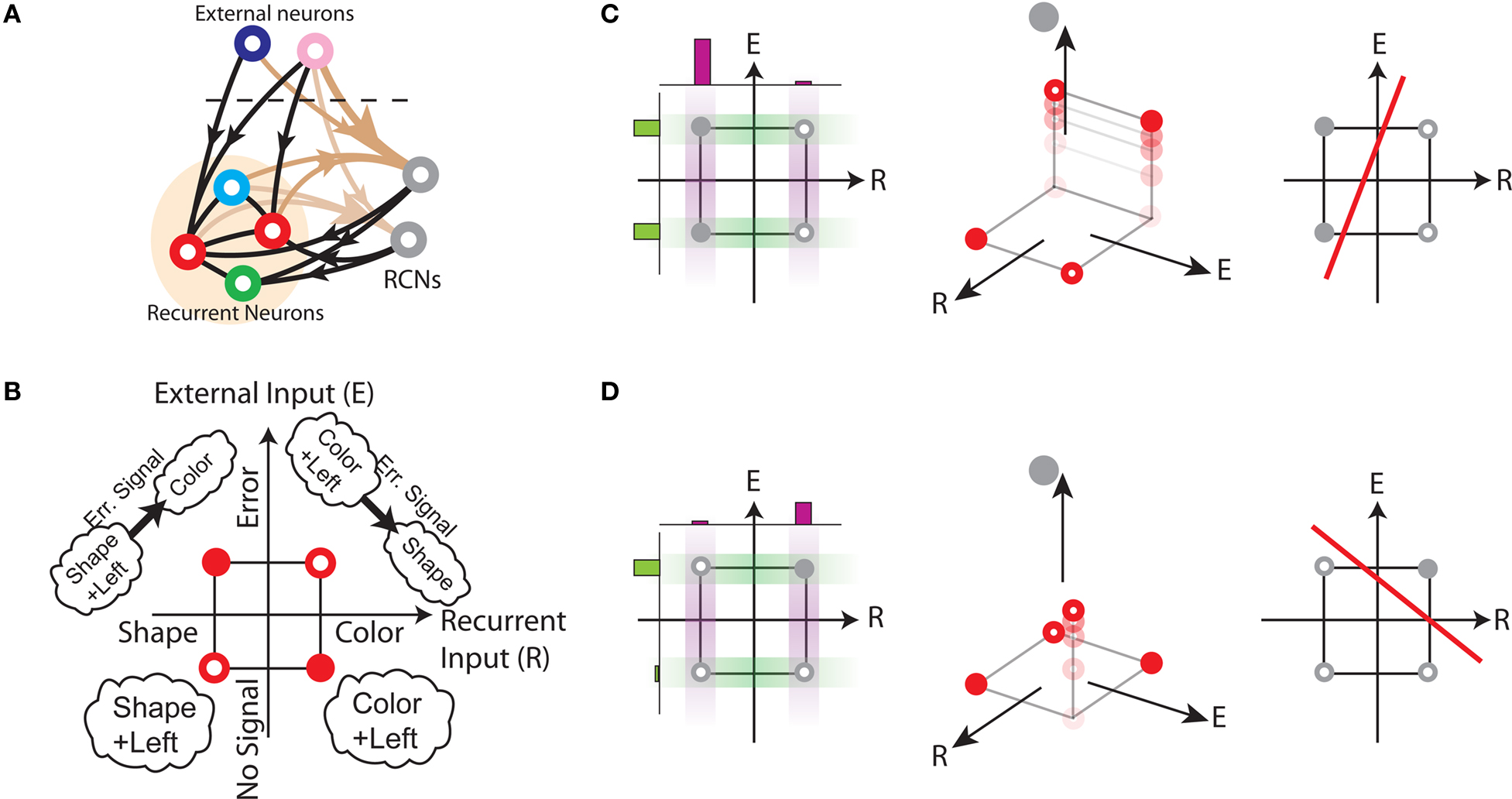
Figure A1. (A) Architecture of the network, reproduced from Figure 2 for convenience. (B) The context dependence problem is equivalent to the XOR (exclusive OR problem). The N-dimensional space of all possible inputs is projected onto the plane described in the text. The circles represent the desired output activity of a specific neuron (in our case a red, Color Rule encoding neuron) in response to the input identified by the location of the circle on the plane. The desired outputs are dictated by the requirements of the conditions corresponding to the attractors (lower quadrants) and the event-driven transitions (upper quadrants). (C) Effects of an additional neuron with pure selectivity to the inner mental states. Left: the neuron (gray) responds to two of the four possible inputs (leftmost points) and hence it has pure selectivity. The response to the two inner mental states (Shape + Left, Color + Left) averaged over the two possible external inputs is represented by two bars above the square. The response to the external inputs averaged over the inner mental states is plotted vertically and it is represented again by two bars. The neuron responds differently and is selective to the inner mental states but not to the external inputs. Center: effects of the introduction of the pure selectivity neuron in the network dynamics. The input space goes from a plane to the third dimension, spanned by the activity of the additional neuron. Two of the circles representing the outputs of the Color Rule neurons (see B) move up to reflect the activity states of the additional neuron. The axes directions are correct, but their position is arbitrary. Right: an RCN with pure selectivity responding to the same input space represented in (B). The position and orientation of the red line is determined by the random synaptic weights. For this particular realization separates two inputs on the left, which are the input patterns activating the RCN. (D) Same as in (C) but for a mixed selectivity neuron.

We now consider the most general case and we denote by ẖ⁰ the vector of the activities of the external neurons in the absence of events, and by ẖ¹, the pattern of activity corresponding to the occurrence of E. The input patterns are N-dimensional activity vectors where N is the total number of neurons on a dendritic tree. Whenever we have the non-linear separability problem described above, the four input patterns are constrained to lie on a plane that is spanned by two vectors: (1) one along the direction of inner mental state selectivity, e.g., [,ẖ⁰] − [,ẖ⁰], and (2) one along the external input selectivity, e.g., [,ẖ¹] − [,ẖ⁰]. Figure A1B shows a representation of such a plane. The projections of the four possible inputs onto the plane lie at the vertices of a rectangle (in our specific example, a square), where we placed four red circles. The position of the rectangle with respect to the axes will in general depend on the vectors ,ẖ^0,1. We chose a simple symmetric case in which the axes cross at the center of the rectangle. The filling colors of the circles represent the desired output activity of one particular neuron of the recurrent network. In our specific case it is the output of a neuron representing Color Rule, when we impose the four conditions corresponding to the attractors and the Error Signal driven transitions indicated in the figure. For example, when we impose that Color + Left is an attractor (lower right), the neuron should be active, and this is represented by a filled circle. The Error Signal should trigger a transition to Shape and hence inactivate the neuron (empty circle in the upper right quadrant). The output of our particular neuron is a XOR of the Color-Error Signal neuron activities. The fact that there is no set of synaptic weights implementing this function translates graphically in the impossibility of finding an hyperplane (a line on the projection plane) separating the inputs that should activate the Color neuron from those that should inactivate it.

The probability of not encountering the context-dependent problem is exponentially small for random uncorrelated patterns

The probability that such a situation occurs depends on the statistics of the patterns representing the mental states, and on the set of event-driven transitions. We now compute the probability that the conditions for attractors and transitions cannot be imposed simultaneously when the attractor patterns are random and uncorrelated and the neurons are active with probability 1/2. Given one particular event occurring in two contexts corresponding to two attractors, the probability that it generates a non-linear separability on one output neuron, is 1/8. Indeed, there are two possible outputs for each of the four input patterns (two attractors and two transitions), for a total of 2⁴ = 16 possible input–output relations. For two of them (the XOR, and its negation) the patterns are non-linearly separable. As there are N output neurons, the probability that the patterns are linearly separable for all outputs is

which goes to 0 exponentially with N. If the number of contexts C in which the same event occurs is more than 2, then the exponent is proportional to NC. Notice that the probability that the problem is solvable decreases as N increases.

It therefore turns out that the case of random uncorrelated patterns, which requires a simple learning prescription for attractor neural networks (Hopfield, 1982; Amit, 1989), becomes extremely complicated in the case of attractors and event-driven context-dependent transitions. On the other hand, correlations between patterns might reduce the performance degradation, as they could decrease the probability that the same event modifies in two different directions the activity of a particular neuron.

The Importance of Mixed Selectivity

Mixed selectivity and context dependence

The problem of non-linear separability described in the previous Section can be solved by the introduction of neurons with mixed selectivity that participate in the network dynamics. We first show in Figure A1C that additional neurons with “pure selectivity” either to the inner mental state or to the external input cannot solve the problem. Then, in Figure A1D, we show that there is always a solution when we introduce a mixed selectivity neuron in the network. Such a solution can be implemented as a network of RCNs (Figure A1A).

Consider a neuron that is selective to the mental states, i.e., when its average response to the inputs containing , (i.e., [,ẖ⁰] and [,ẖ¹]), is different from the average response to the inputs containing . The left part of Figure A1C shows one example of a neuron that is selective to the mental state, but not to the external input. The input space is represented as in Figure 1B, and we now consider the output of an additional neuron that activates when in Shape + Left mental state, but not in Color + Left, regardless of the external input. Active outputs are indicated by filled gray circles.

When we introduce such a neuron in the network, the N-dimensional input space becomes N + 1 dimensional. We can observe the effects on the Color Rule neuron of the embedding in a higher dimensionality in the middle part of Figure A1C. The extra dimension introduced by the additional neuron is along the z-axis, and the plane of Figure A1B is now spanned by the x and y axes. Two of the circles now move up to reflect the activation of the additional neuron when the network is in the Shape + Left mental state. Unfortunately, this new placement still does not allow us to draw a plane that separates the inputs activating the Color Rule neuron from those that inactivate it. This shows that “pure selectivity neurons” do not solve the non-linear separability problem. The rightmost plot will be explained in the next section.

Consider now the mixed selectivity neuron of Figure A1D. Such a neuron is selective both for the mental states and the external input, as shown by the leftmost plot of Figure A1D. Now the embedding in a higher dimensional space can allow us to solve the problem, as only one circle moves up in the central plot of Figure A1D. It is easy so see that it is possible to draw a plane that separates the two empty circles from the filled ones. For similar geometrical considerations, we can conclude that the problem of non-linear separability can be solved for all additional neurons that respond to an odd number of the four possible inputs. Notice that there are two situations in which moving an even number of circles would also solve the problem (when the opposite circles move up or down). However these situations cannot be realized by a single neuron, as it would implement a non-linear separable function.

The general importance of mixed selectivity

To show the general importance of mixed selectivity we consider, for simplicity, binary neurons that can be either active or inactive. Each neuron can be regarded as a unit that computes a Boolean function φ(·) of the vector of the N activities s₁,…,s_N of the synaptically connected input neurons, which include the recurrent and the external neurons (s = {0,1}). The problem of context-dependent tasks is related to the fact that the class of Boolean functions that can be implemented by a neuron is restricted, as it is usually assumed that the neural response is a monotonic function of the weighted sum of the activities of the synaptically connected neurons. More formally, consider a McCulloch–Pitts model neuron that is described by

where J_ij is the synaptic efficacy of the coupling between neuron j and neuron i, Θ is the Heaviside function [Θ(x) = 0 if x ≤ 0, Θ(x) = 1 otherwise], and θ is the activation threshold. Different sets of synaptic efficacies correspond to different Boolean functions. How does the set of functions implementable by a McCulloch–Pitts neuron compare to more general Boolean functions, which would include also the ones that solve context-dependent problems? It is illuminating to expand a general Boolean function in a series of terms containing products of the input variables (Wegener, 1987):

where the Cs are the coefficients of the expansion. Such an expansion is similar to the Taylor expansion of a function of continuous variables, although in the case of Boolean functions the number of terms is finite and equal at most to 2^N. Every term is either a single variable, or a product of two or more Boolean variables. This is equivalent to performing the logical OR operation (sum in the expression) of logical ANDs (products) between variables.

A McCulloch–Pitts neuron reads out a weighted sum of the activities s₁,…,s_N, and can therefore only implement Boolean functions that depend on the first order terms of the expansion. The coefficients C_ij are equivalent to the synaptic weights J_ij of the neuronal inputs. Equation 7 suggests that, in general, we may need to consider also higher order terms to solve complex problems.

Notice that each term taken singularly, or the sum of terms of the expansion can be considered as the output of an additional neuron that responds to a particular combination of generic events according to Eq. 6. Each C can be then regarded as the synaptic efficacy of the connection from such a neuron to the output neuron s_i. For example, the term C_i12s₁s₂ can be interpreted as the input to neuron s_i from a neuron that is active only when both s₁ and s₂ are active, with the synaptic strength C_i12. The neuron of Figure 2B, that solves the problem of context dependence by responding to the Error Signal only when starting Shape Rule, actually implements one of these higher order terms.

Estimating the Number of Needed RCNs

Single context dependence: a graphical analysis

The prescription we use to create Randomly Connected Neurons (RCNs) leads to neurons with mixed selectivity. What is the probability that an RCN solves the problem generated by one particular context-dependent transition? In order to solve the problem, we showed in Section ‘The importance of mixed selectivity’ that the “ that the neuron should have mixed selectivity, or in other words, in our paradigmatic example, the neuron has to respond to an odd number of the four possible input patterns [,ẖ⁰], [,ẖ¹], [,ẖ⁰], [,ẖ¹]. What is the probability that an RCN has such a response property? The RCN is active if the weighted sum of its inputs ν_j is above some threshold θ:

where the K_j’s are the synaptic weights and the sum extends over both the external inputs and the neurons of the recurrent network. Choosing a specific set of synaptic weights and a threshold is therefore equivalent to drawing an hyperplane in an N-dimensional space (whose equation is Σ_jK_jν_j = θ) that separates the input patterns activating the RCN from those that don’t activate it. For some of these hyperplanes, the RCN implements the mixed selectivity neuron that we need in order to solve the context dependence problem of Section ‘Constraints on the types of implementable context-dependent transitions’. Consider for simplicity the case N = 2, in which the activity patterns lie on a plane. In this case, the problem amounts to determining a set of synaptic weights and a threshold so that the line has a particular orientation and displacement with respect to the origin. The rightmost part of Figure A1C shows how an RCN responds to the four possible input patterns [,ẖ⁰], [,ẖ¹], [,ẖ⁰], [,ẖ¹], that lie on the same plane introduced in Figure A1B. The RCN output is determined by the orientation of the red line that represents one realization of the random synaptic weights. The gray circles on the left of the line indicate that the neuron is activated by Shape + Left, no matter what is the value of the external input. Such a neuron has “pure” selectivity and it does not solve the non-linear separability problem. The second example in Figure A1D, shows an RCN connected by a different set of synaptic weights. The orientation and placement of the red line isolate only one vertex of the square, and the RCN shows mixed selectivity. In this second case, the introduction of this RCN solves the non-linear separability problem. What is the probability that an RCN has this kind of mixed selectivity?

Random synaptic weights would imply random orientation and displacement with a distribution that depends on the dimensionality of the original space of input patterns (N), on the statistics of the random weights and on the threshold for neuronal activation. In our case the probability of drawing a particular line is isotropic with respect to the origin (see probability density function in Figure A2A) and depends only on the distance from the center of the square. In particular, it grows to a maximum and then it decays to 0 (see Figure A2C). The only useful RCNs correspond to those that isolate a single vertex. Those lines that are far from the center of the square do not cut any edge joining two of the four input patterns, and they do not solve the non-linear separability. As a consequence, the best distributions are those localized around the center of the square, as in the case of Figure A2B, i.e., for small thresholds θ. In all these situations the fraction f of all possible patterns of the input space that activate the RCN is close to 1/2, whereas, when the threshold θ is large, f tends to 0.

FIGURE A2

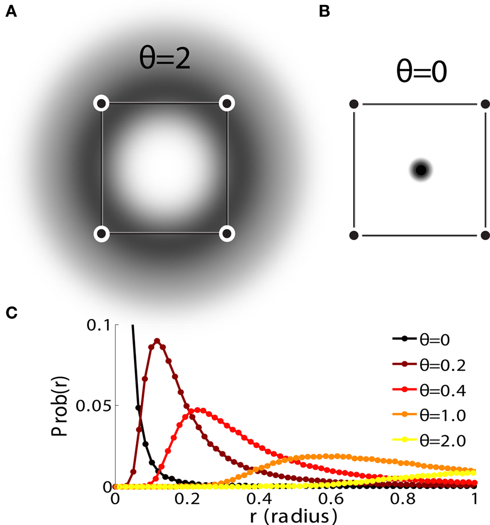
Figure A2. (A) Density of circles tangent to the planes generated by randomly sampling RCNs with Gaussian synapses and θ = 2. (B) Same as (A), but with θ = 0. (C) Distribution of the radii of tangent circles for different values of the firing threshold θ.

We now give a more general and formal explanation for the importance of the kind of mixed selectivity we introduced in our network. We seek to prove that as the number of RCN grows, the probability to be able to implement an arbitrary scheme of attractors and transitions goes to 1. We first analyze two specific cases, the ultra-sparse case in which f is very small and every RCN responds to only one input pattern, and the dense case in which f = 1/2.

The ultra-sparse case

In the case in which the RCNs are connected to the neurons of the recurrent network by random binary synapses, we can tune the neuronal threshold such that f = 1/2^N, i.e., every RCN is activated by a single input pattern. In such a case every additional unit generates one term of a particular Boolean expansion, known as the Disjunctive Normal Form (Wegener, 1987). Using the same notation as in Section ‘The importance of mixed selectivity’, we can write the activity of a generic neuron s_i of the recurrent network as:

s_i(t + 1) = φ_i(s₁(t),…, s_N(t)) = θ(C_i1s₁(t)(1 − s₂(t)),…, (1 − s_N(t)) + C_i2s₁(t)s₂(t)(1 − s₃(t)),…, (1 − s_N(t))+…),

where Θ is the Heaviside function and the Cs are the coefficients of the expansion. Every term is a product of some Boolean variables and the negation of the others (which is one minus the original variable). If these neurons are part of the recurrent network, then they can also be considered as input neurons and can contribute to the total synaptic current. If we choose the proper synaptic weights and have enough RCNs, we know that we can generate any arbitrarily complex function of the inputs s₁,…,s_N. This is an extreme case in which the number of needed RCNs grows exponentially with the number N of neurons in the recurrent network. However, in such a case, not only we can satisfy all possible conditions for the attractors and the event-driven transitions, but in principle we can also shape the basins of attractions arbitrarily.

The general case (any coding level) for single context dependence

We consider the paradigmatic case of a single context dependence as the one described in Section “Constraints on the Types of Implementable Context-Dependent Transitions.” Our aim is to compute the probability that an RCN solves the context dependence problem. We will show that this probability depends on the sparseness of the representations of the mental states, the external inputs and the corresponding patterns of activities of the RCNs. The main result of this paragraph will be that the maximum will always be in correspondence of dense representations.

In order to solve the non-linear separability due to the context dependence problem, we need an RCN that responds to an odd number of the four possible input patterns [,ẖ⁰], [,ẖ¹], [,ẖ⁰], [,ẖ¹] (mixed selectivity).

We consider one particular randomly connected neuron (RCN) and calculate the probability that it responds as a mixed selectivity neuron. Our RCN, whose activity level we will denote by the binary variable η (for now η = −1 or 1 for simplicity, but see below for the other cases), receives inputs from both internal and external excitatory neurons with synapses independently and identically sampled from two distributions with finite first and second moments equal to 〈K^r〉 = μ_r and , and 〈K^x〉 = μ_x and , respectively.

We assume that the statistics of these synapses is independent from that of the patterns. The activity η depends on the total synaptic input and the firing threshold, denoted with θ:

where the and factors have been introduced to keep the total synaptic current intensive.

We now calculate the coding level of the RCN, that is, the probability that η is positive.

Coding level of the RCN network. Assuming a large number of pre-synaptic recurrent and external neurons (N_r,N_x → ∞) we can harness the central limit theorem to calculate the terms contributing to the synaptic input to η in Eq. 9. The following quantities are distributed according to a normal distribution as follows:

We can then calculate the coding level of one RCN as a function of the firing threshold θ:

with , and where we used the standard definition of the error function: and erfc(x) = 1 − erf(x). The coding level of the RCN network is therefore given by:

Conversely, in order to obtain RCNs with a given coding level f we can set the firing threshold to be:

where with erfc⁻¹ we indicate the inverse function of erfc, i.e., the function for which erfc⁻¹(erfc(x)) = x.

RCNs and linear separability. We now calculate the probability p that a particular RCN η responds only to an odd number of cases, that is when all but one of the terms η(ξ¹,h⁰), η(ξ²,h⁰), η(ξ¹,h¹), η(ξ²,h¹) are the same. To calculate this probability we start by defining the following three independent random variables:

where the sum is over all the indices j for which , and so on. With these definitions we can explicitly write down the activity of η in the four conditions in the following way:

η(ξ¹,h⁰) = sign(g₊ + g_r + g_x), η(ξ¹,h¹) = sign(g₊ + g_r − g_x),

η(ξ²,h⁰) = sign(g₊ − g_r + g_x), η(ξ²,h¹) = sign(g₊ − g_r − g_x).

The quantities defined in Eqs 11 and 12 are independent Gauss distributed variables whose variance depends on the correlations (overlaps) between the patterns ξ, h representing the mental states and the external stimuli. Let us denote with o_r the overlap between ξ¹ and ξ², and with o_x the overlap between h⁰ and h¹:

Note that the overlaps o_r,o_x are quantities between −1 and 1.

Using the fact that and the analogous identity for N_x it is simple to verify that g_r,_x,+ are distributed in the following way:

where we have used the following definitions

Note that , are quantities between 0 and 1 quantifying how similar ξ¹ is to ξ² and h⁰ to h¹, respectively. As a matter of fact is equal to 0 if ξ¹ is totally anti-correlated to ξ² (that is ξ¹ = −ξ²), is equal to 1 if ξ¹ is equal to ξ², and is equal to one half for the intermediate case of uncorrelated patterns.

We can now calculate the probability p that one of the η’s has an opposite sign with respect to all the others. Taking into account the distributions of the variables given in Eq. 14 this probability is given by:

where with (x ↔ r) we indicate a summand equal to the previous term in Eq. 16 with the only difference that x and r indices have to be exchanged.

We now consider the case in which the patterns representing the mental states and the external events have the same statistics. We therefore assume that o_r = o_x = o, which implies that . We also assume without loss of generality that . Equation 16 then simplifies to

For the special case of random uncorrelated patterns with coding level f₀ = 1/2 we have that o_r = o_x = 0, which means that . In this case, Eq. 17 further simplifies to:

Maximizing the probability of linear separability for random patterns. We now want to further examine the case in which mental states and external stimuli are represented by uncorrelated random patterns with coding level f₀ = 1/2. This is the simplest maximal entropy situation which is also the most commonly investigated in the computational literature. The probability p of linear separability for random uncorrelated f₀ = 1/2 patterns is given in Eq. 18. This expression is clearly symmetric in θ and can be shown to have a maximum at θ = 0. For this case corresponding to dense coding f = 1/2 we therefore have a maximal probability which can be calculated to be

meaning that on average one additional mixed selective unit out of three will be useful to solve the context dependence problem. This is a surprisingly high fraction, considering that the representations and the synaptic connections to the RCN are completely random.

Figure A3 shows the probability p of finding a mixed selective RCN as a function of the RCN’s firing threshold for different values of the overlap o. As it can be seen, for positive o the maximum is always at θ = 0 which corresponds to dense coding level f = 1/2. Moreover, increasing the overlap o decreases the probability of finding mixed selective RCNs. This can be intuitively understood considering that an increasing value of o corresponds to an increasing similarity between the patterns, and therefore an increasing difficulty to linearly separate them. Notice that the case of positive overlap o can always be led back to a case of random uncorrelated patterns with a coding level f₀ satisfying o = (2f₀ − 1)². Conversely, the case of random patterns with coding level f₀, corresponds to the case of positive o = (2f₀ − 1)².

FIGURE A3

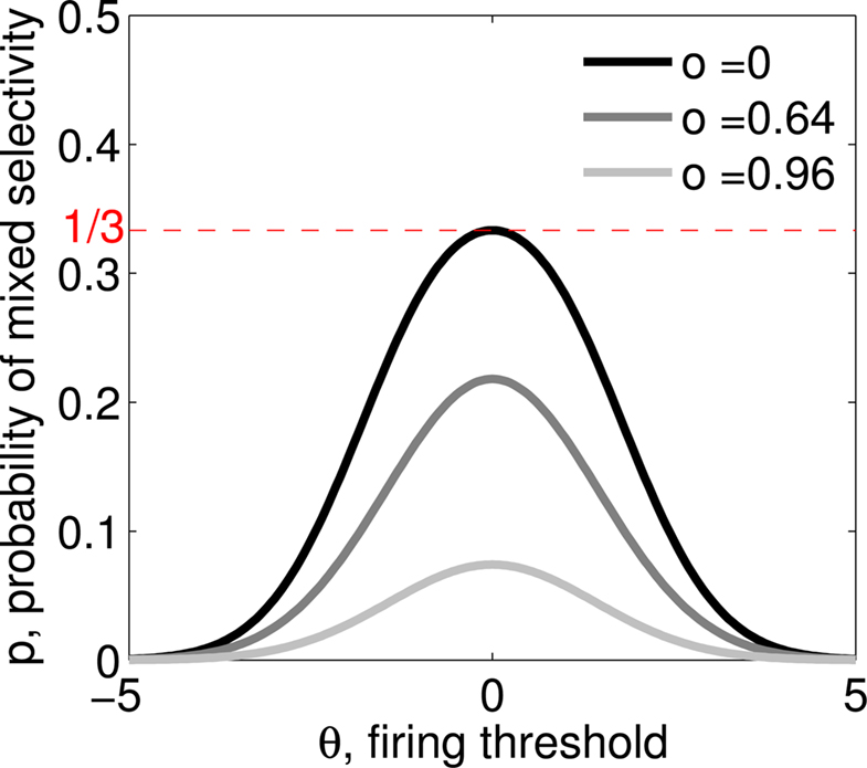
Figure A3. Probability of finding an RCN which implements mixed selectivity, therefore allowing to linearly separate the input patterns as a function of the RCN’s firing threshold θ. This quantity is calculated in Eq. 17. Different curves correspond to different positive values of the overlap o of the input patterns representing the mental states and the external events.

Maximizing the probability of linear separability for anti-correlated patterns. We now want to consider the case in which we are allowed to manually pick the patterns representing the mental states and the external stimuli. In particular, let us see what happens if we are allowed to choose anti-correlated patterns, that is pairs of patterns which have a negative overlap o.

Following last paragraph’s intuition we would expect that increasingly negative overlaps push the activity patterns further apart, therefore making them easy to linearly separate. From Figure A4 we see that this is exactly what happens initially for all values of θ and in particular for θ = 0. When o is decreased below 0 the value of p increases for all values of θ, and θ = 0 always corresponds to the maximal value.

FIGURE A4

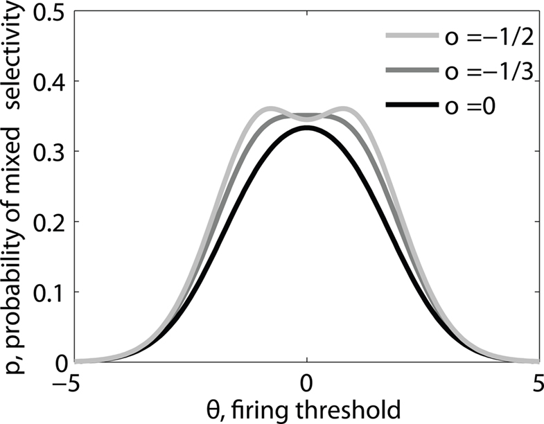
Figure A4. Probability of finding an RCN which implements mixed selectivity as a function of the RCN’s firing threshold θ. This figure is analogous to Figure A3, with the difference that different curves correspond to different negative values of the overlap o of the input patterns representing the mental states and the external events.

This trend crucially stops at a critical value of o = −1/3. Below this point, the value of p at θ = 0 starts to decrease and Figure A4 shows that the maxima of the value of p shift laterally to θ ≠ 0.

It is possible to calculate analytically the critical value o = −1/3 of maximal p for θ = 0 maximizing the expression in Eq. 17. First of all let us compute the value of p at θ = 0 from Eq. 17:

where we defined . The plot of this expression gives the graph in Figure A5. To find the maximum we have to calculate the extremal points in o by computing the derivative and setting it to 0. Because of the chain-rule:

From the definitions of and Σ the first two factors in Eq. 20 simply give:

Because the derivative of erf is just a Gauss function which is easily integrated, also the third term in Eq. 20 results in a fairly simple expression:

Putting the last three equations together we obtain:

which is 0 only for Σ² = 2, that is for , which in turn corresponds to o = −1/3. This in fact is the maximum point which can be graphically inferred from Figure A5.

FIGURE A5

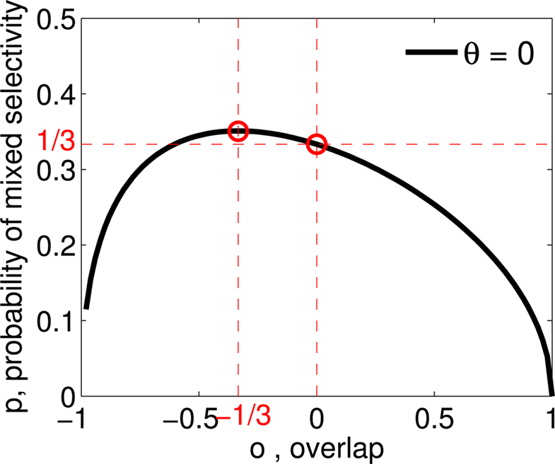
Figure A5. Probability p of finding an RCN implementing mixed selectivity as a function of the overlap o between the input patterns for a constant value of the RCN firing threshold θ. We see that by going to negative o we can slightly increase p until a value o = −1/3. At this point θ = 0 stops being a maximum of p.

We now consider what happens for values of the overlap o which are even more negative than o < −1/3. This is illustrated in Figure A6.

FIGURE A6

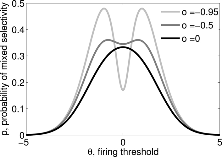
Figure A6. Probability of finding an RCN which implements mixed selectivity as a function of the RCN’s firing threshold θ. Different curves correspond to different negative values of the overlap o of the input patterns representing the mental states and the external events.

The value of p at θ = 0 goes to 0 as o → −1 and the maximum monotonically increases and shifts away from θ = 0. We can therefore ask two questions.

First of all, what is the value of the absolute maximum which is reached at o = −1? Derivation and numerical integration of the expression (Eq. 17) for this case shows that this maximum is p_max = 0.5.

The second question we can ask is, how fast does the value of p go to 0 as o approaches −1? To calculate how fast p goes to 0 as o goes to −1 let us recall that the quantity is a measure of how different the pattern ξ¹ is from ξ² and h⁰ is from h¹, and is exactly equal to 0 for totally anti-correlated patterns. We therefore want to Taylor-expand expression (Eq. 17) at θ = 0 around , that is for the case of anti-correlated patterns.

To do this we can use Eqs 21 and 22 together with the fact that

which gives:

This means that in the θ = 0 case for very anti-correlated patterns, that is for , the probability of finding a useful RCN goes to 0 as the square root of :

We can also compute how fast p goes to 0 when the input patterns are increasingly similar, that is for the case o → 1, corresponding to . This gives the same type of decay:

In conclusion, we have seen that the case θ = 0 corresponding to a dense RCN coding level f = 1/2 always gives the highest probability p to obtain a useful RCN. The only regime for which the case θ = 0 is not the most favorable one is when we are allowed to choose anti-correlated patterns with an overlap below o = −1/3. Nonetheless, the probability at θ = 0 decreases relatively slowly when we depart from the random uncorrelated case o = 0. Notice that the best possible value of p which is obtained by choosing ad hoc the input patterns is p_max = 0.5, which is a relatively small gain with respect to the value p_max =1/3 which we get for purely random input patterns.

From ±1 to 0/1 neurons

All the conclusions illustrated in the previous sections are easily translated to the case in which we represent the neuronal activity with Boolean variables (0/1), rather than ±1 variables. We show this by first introducing the relation between the ±1 variable ξ to the 0/1 Boolean variable :

Equation 9, defining the activity of an RCN, can then be translated to the Boolean case as follows:

where Θ(·) denotes the Heaviside’s step function: Θ(x) = 1 if x > 0, and Θ(x) = 0 otherwise. Equation 23 can be rewritten as:

by defining as a random variable with mean and variance , and as a random variable with mean and variance . Finally μ_i is a constant inhibitory current

These equations show that switching from a ±1 to a 0/1 representation, is equivalent to modifying the statistics of the random synaptic connections, and introducing an additional inhibitory term. This simple consideration provides us with a straightforward way to extend the results of the analysis of ±1 neurons to the case of 0/1 neurons. Indeed, it is easy to generate Boolean 0/1 RCNs with the same statistical properties as the ±1 RCNs that we considered in the previous paragraphs. Assume for instance that we are given an ensemble of Boolean 0/1 RCNs whose activity is described by Eq. 24 with synapses independently drawn from a distribution with finite first and second moments equal to and and and , respectively. The statistics of the firing patterns of these RCNs, and in particular the probability the coding level f and the probability that an RCN has mixed selectivity, will be the same as the statistics of the ±1 RCNs of Eq. 9, provided that the first and second moments of the synapses are properly rescaled by a constant factor. In particular, when and have finite first and second moments equal to and , and and , respectively. As a result, the coding level of the Boolean RCN in Eq. 24 (that is, the fraction of pre-synaptic configurations for which the neuron is active, i.e., its activity is not 0) is given by translating Eq. 10 to the Boolean “hatted” variables:

In other words, this equation gives the coding level f of a Boolean 0/1 RCN whose activity is described by Eq. 24, with synapses independently drawn from a distribution with finite first and second moments equal to and , and and , respectively.

The remaining equations of the last sections are also easily translated from ±1 variables to Boolean variables. In order to do that we introduce the following definitions for the overlaps corresponding to Eq. 13:

where indicates the “negation” of the Boolean variable ξ, i.e., . Note that from Eqs 13 and 26 it is easy to see that:

consistently with the definitions in Eq. 15.

This set of simple relations between “hatted” and “unhatted” variables allows us to translate the results obtained in the previous paragraphs for the case of ±1 coding neurons to the case of 0/1 neurons. For instance, the graphs in Figure A3, where we normalized the synapses so that , would correspond in the 0/1 coding case to a normalization . With this set of parameters and using Eq. 27 to convert the overlaps o_r, o_x in the ±1 case to the overlaps , in the 0/1 case, we can see that the plots corresponding to o = 0,0.64,0.96 would be translated in the 0/1 coding scheme to overlaps between the patterns of respectively. A similar conversion can be easily carried out for the other results illustrated in Figures A4–A6.

Similarly, when the probability that an RCN has mixed selectivity is plotted against f (the coding level of the RCNs), the curves are the same in the ±1 as in the 0/1 case, although each point is characterized by a different set of parameters in the two cases (in particular the statistics of the synapses and the threshold). As a consequence, f₀ (coding level of the input patterns) and the overlap o indicated in the plots and characterizing different curves, should be recalculated as explained above. All the considerations about the position and the value of the maximum discussed in the main text remain unchanged when the 0/1 case is considered.

The dense case: multiple context dependencies

What is the total number of RCNs needed to satisfy all conditions corresponding to a large number of transitions and stationary patterns of neural activity? Were all context-dependent transitions independent, such a number would be proportional to the logarithm of the number of conditions. This is certainly true for a small number of context-dependent transitions. Unfortunately, the conditions to be imposed for a large number of context-dependent transitions are not independent, and an analytic calculation turned out to be rather complicated.

Hence we devised a benchmark to characterize numerically the scaling properties, in simulations where transitions between randomly selected attractors were all driven by a single event. Half of the m mental states were chosen as initial states, i.e., the contexts in which the event can occur. For each initial state we chose randomly a target attractor. The representations of the attractors were random uncorrelated patterns. Figure A7A shows the required number of RCNs as a function of the number of transitions that are needed in a task. The average number of necessary RCNs scales logarithmically with the number of contexts m for small m values, and then linearly. Moreover, the minimal number of RCNs is achieved for f = 1/2, consistently with the full simulations of Figure 5A. The required number of RCNs increases with decreasing f, approximately like 1/f when f ≤ 1/2 (see Figure A7B), and like 1/(1 − f) for f > 1/2 (not shown). Notice that in Figures A7A,B we plotted the number of needed RCNs for satisfying the mathematical conditions that guarantee the stationarity of the patterns of activities of the mental states and the implementation of the event-driven transitions. When we additionally require that the stationary points are stable and the basin of attraction has a given size, as in Figures 5B,D the situation is significantly worse in the case of f ≠ 1/2, but the scaling with the number of mental states remains linear.

FIGURE A7

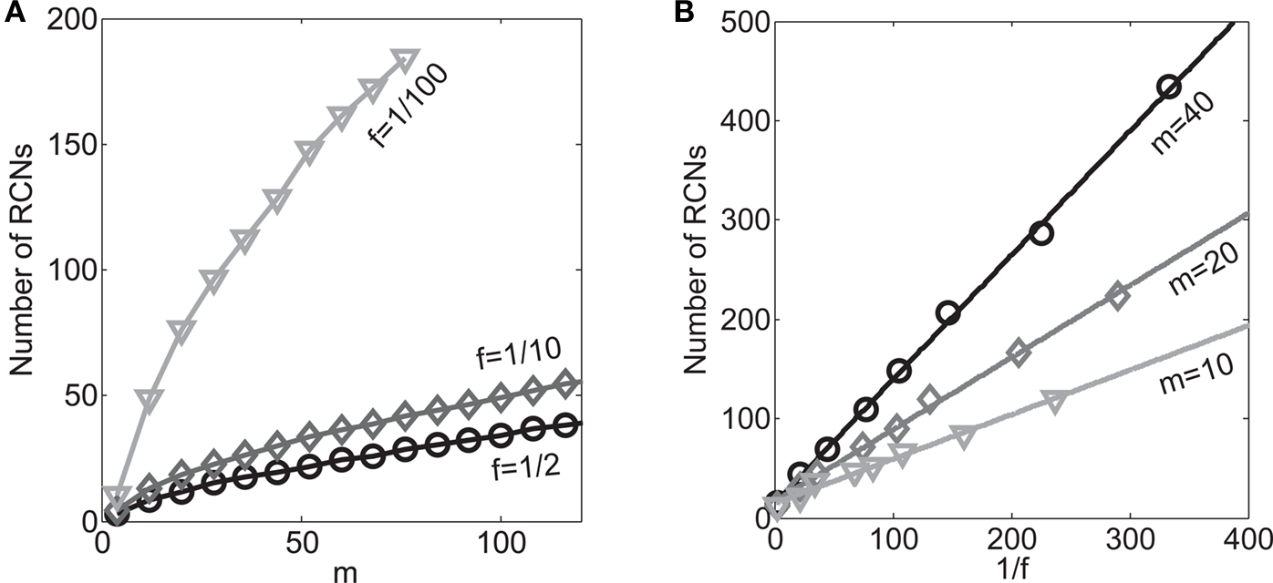
Figure 7A. (A) Number of RCNs needed to implement m/2 transitions between m random mental states. The number of neurons in the recurrent network is always N = 200. Different curves correspond to different choices of the threshold for activating the RCNs, which, in turn, correspond to a different f (average fraction of inputs that activate the RCNs). (B) Number of needed RCNs as a function of 1/f for a different m. N = 200 as in (A).

The Number of Learning Epochs Decreases with the Number of RCNs

When RCNs are added to the network, not only the neural patterns of activity become linearly separable, but they also become more separated. Indeed, adding RCNs to the network is equivalent to embedding the neural patterns representing the mental states into a higher dimensional space. Although the relative distances between different patterns are approximately preserved, the absolute distances increase with the number of RCNs, increasing the separation between the neural patterns that should produce active neurons from those that are supposed to produce inactive neurons. One consequence of this is that it becomes easier to find a hyperplane separating these two classes of patterns, and hence the number of learning epochs required by the perceptron algorithm decreases, as predicted by the perceptron theorem (Block, 1962). The phenomenon is illustrated in Figure A8, where we plotted the average number of learning epochs required to satisfy all conditions to realize the attractors and transitions, as a function of the number of RCNs. This was done for three different numbers of attractors and transitions. The number of learning epochs decreases rapidly as RCNs are added to the network. Although this is not the real learning process used by the brain (here we assume that the set of mental states and transitions are already known), it gives strong indication that our network has the highly desirable property that learning becomes simpler and faster as the number of RCNs increases.

FIGURE A8

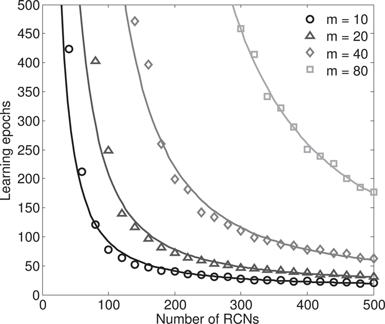
Figure A8. The number of required learning epochs decays as the number of RCNs increases for a fixed minimal stability parameter γ = 0.5. The number of epochs is plotted for four different levels of capacity (m = 10,20,40,80). The solid lines are the power law curves fitted to the datapoints (the power ranges from approximately −1.5 to −2.2 as m increased). The asymptotic number of learning epochs seems to increase lineary with the number of transitions and the number of attractors m, ranging from approximately 12–40 (not visible in the plot), for m = 10 and 80, respectively. Parameters as statistics of the neural patterns are as in Figure A7.

Stochastic Transitions Between Mental States

In the simulations illustrated in Figure 6 the transitions induced by the external events are deterministic. However, if in Eq. 5 we increase the noise in the neural activity, they can become stochastic, occurring with a probability that depends on the noise amplitude σ, and on the stability parameter γ used in the perceptron algorithm to compute the proper synaptic couplings (see Eq. 2). Different conditions, corresponding to different attractors or event-driven transitions can be imposed with a different strength depending on the stability γ used during learning. Even in the case in which the stability parameter is always the same, there might be differences in the implemented conditions, due to correlations between the representations of the mental states and to particular structures in the scheme of transitions. For example in the case of the simulations of Figure 6, the transitions between one rule to another, induced by the Error Signal are the weakest, and the most vulnerable to noise. Indeed as the level of neural noise increases, these transitions become stochastic and progressively less probable, as illustrated in Figure A9. Notice that the other transitions occurring within each trial remain unaffected. The decrease of transition probability is due to the fact that the external input is required to drive the recurrent and the randomly connected neurons consistently in one particular direction for the entire duration of the event triggering the transition. Noise makes the driving force stochastic, inconsistent, and overall weaker, thus reducing the chances that the transition will occur. As the starting mental state is an attractor of the dynamics, the network will return to the initial state. This is an important property of the network, as sometimes it is required to have transitions that occur with some probability, as in the case of an uncertain environment. Moreover stochasticity is fundamental for the latching dynamics, i.e., the ability of the neural circuit to jump spontaneously from one mental state to another (Kropff and Treves, 2005; Treves, 2005). Latching dynamics has been extensively discussed for its importance in cognitive processes related to language.

FIGURE A9

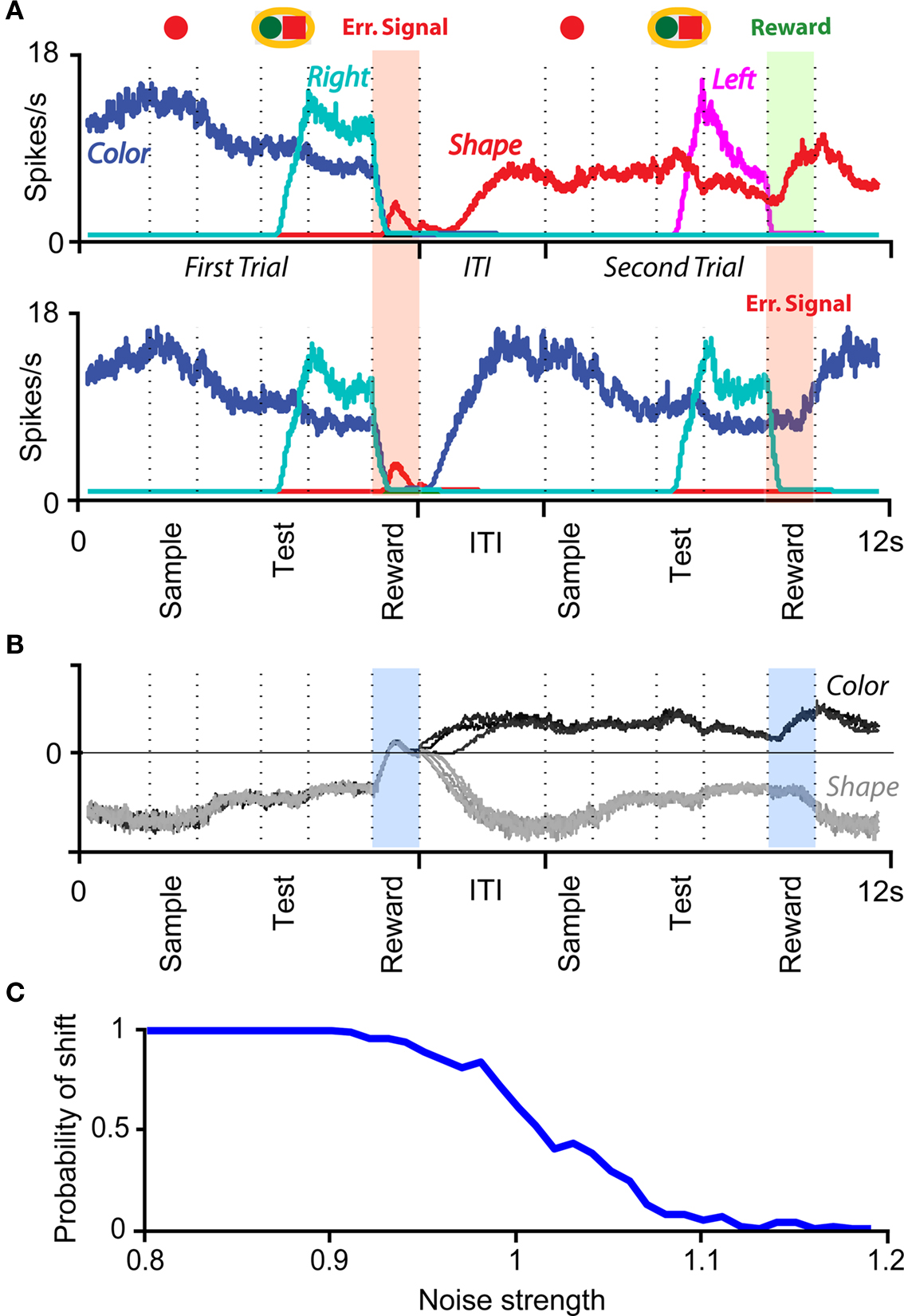
Figure 9A. Stochastic event-driven transitions. A larger amount of noise is injected in the simulated neurons of Figure 6. The transitions between the two mental states corresponding to the rules become stochastic. (A) The neural activity of four highly selective neurons (to color rule, shape rule, touch left, and touch right) is plotted as a function of time. In the top panel the absence of reward induces a transition from one rule to the other, whereas in the bottom panel, under the same conditions, the transition does not occur. (B) Difference in activity between two neurons selective to shape and color rule, respectively, for several occurrences of the Error Signal event. In half of the case the transition occurred, and in the other half it did not. (C) Probability of completing a transition as a function of normalized noise (noise strength is defined as unitary in correspondence to a 1/2 transition probability).

Conflict of Interest Statement

The authors declare that the research was conducted in the absence of any commercial or financial relationships that could be construed as a potential conflict of interest.

Acknowledgments

We would like to thank O. Barak, E. Curti, G. Hinton, M. Mattia, and S. Seung for useful discussions. We are grateful to L. F. Abbott, P. Dayan, F. Mansouri, A. Roxin, C. D. Salzman, and K. Tanaka for many useful comments on the manuscript. This work was supported by the SNF grant PP00A-106556, by DARPA SyNAPSE and partly by the Gatsby and the Swartz Foundations. Xiao-Jing Wang was partly supported by NIMH grant 2R01MH062349 and the Kavli Foundation.

References

Ackley, D. H., Hinton, G. E., and Sejnowski, T. J. (1985). A learning algorithm for Boltzmann machines. Cogn. Sci. 9, 147–169.

CrossRef Full Text

Albus, J. (1971). A theory of cerebellar function. Math. Biosci. 10, 25–61.

CrossRef Full Text

Amit, D. J. (1988). Neural networks counting chimes. Proc. Natl. Acad. Sci. U.S.A. 85, 2141–2145.

Pubmed Abstract | Pubmed Full Text | CrossRef Full Text

Amit, D. J. (1989). Modeling Brain Function. New York, NY: Cambridge University Press.

Asaad, W. F., Rainer, G., and Miller, E. K. (1998). Neural activity in the primate prefrontal cortex during associative learning. Neuron 21, 1399–1407.

Pubmed Abstract | Pubmed Full Text | CrossRef Full Text

Barraclough, D. J., Conroy, M. L., and Lee, D. (2004). Prefrontal cortex and decision making in a mixed-strategy game. Nat. Neurosci. 7, 404–410.

Pubmed Abstract | Pubmed Full Text | CrossRef Full Text

Block, H. (1962). The perceptron: a model for brain functioning. Rev. Mod. Phys. 34, 123–135. Reprinted in: Anderson and Rosenfeld (eds.), Neurocomputing: Foundations of Research.

Boettiger, C. A., and D’Esposito, M. (2005). Frontal networks for learning and executing arbitrary stimulus-response associations. J. Neurosci. 25, 2723–2732.

Pubmed Abstract | Pubmed Full Text | CrossRef Full Text

Botvinick, M., and Watanabe, T. (2007). From numerosity to ordinal rank: a gain-field model of serial order representation in cortical working memory. J. Neurosci. 27, 8636–8642.

Pubmed Abstract | Pubmed Full Text | CrossRef Full Text

Brunel, N., and Hakim, V. (1999). Fast global oscillations in networks of integrate-and-fire neurons with low firing rates. Neural. Comput. 11, 1621–1671.

Pubmed Abstract | Pubmed Full Text | CrossRef Full Text

Brunel, N., and Wang, X.-J. (2001). Effects of neuromodulation in a cortical network model of object working memory dominated by recurrent inhibition. J. Comput. Neurosci. 11, 63–85.

Pubmed Abstract | Pubmed Full Text | CrossRef Full Text

Candes, E., and Tao, T. (2004). Near-optimal signal recovery from random projections: near optimal signal recovery from random projections. IEEE Trans. Inf. Theory 52, 5406–5425.

CrossRef Full Text

Cerasti, E., and Treves, A. (2010). How informative are spatial CA3 representations established by the dentate gyrus? PLoS Comput. Biol. 6, e1000759. doi: 10.1371/journal.pcbi.1000759.

Pubmed Abstract | Pubmed Full Text | CrossRef Full Text

Cortes, C., and Vapnik, V. (1995). Support-vector networks. Mach. Learn. 20, 273–297.

CrossRef Full Text

Cromer, J., Roy, J., and Miller, E. (2010). Representation of multiple, independent categories in the primate prefrontal cortex. Neuron 66, 796–807.

Pubmed Abstract | Pubmed Full Text | CrossRef Full Text

Dayan, P. (2007). Bilinearity, rules, and prefrontal cortex. Front. Comput. Neurosci. 1:1. doi: 10.3389/neuro.10.001.2007.

Pubmed Abstract | Pubmed Full Text | CrossRef Full Text

Forrest, B. M. (1988). Content-addressability and learning in neural networks. J. Phys. A Math. Gen. 21, 245–255.

CrossRef Full Text

Funahashi, S., Bruce, C. J., and Goldman-Rakic, P. S. (1989). Mnemonic coding of visual space in the monkey’s dorsolateral prefrontal cortex. J. Neurophysiol. 61, 331–349.

Pubmed Abstract | Pubmed Full Text

Fusi, S., Drew, P. J., and Abbott, L. F. (2005). Cascade models of synaptically stored memories. Neuron 45, 599–611

Pubmed Abstract | Pubmed Full Text | CrossRef Full Text

Fuster, J. M., and Alexander, G. E. (1971). Neuron activity related to short-term memory. Science 173, 652–654.

Pubmed Abstract | Pubmed Full Text | CrossRef Full Text

Ganguli, S., Huh, D., and Sompolinsky, H. (2008). Memory traces in dynamical systems. Proc. Natl. Acad. Sci. U.S.A. 105, 18970–18975.

Pubmed Abstract | Pubmed Full Text | CrossRef Full Text

Genovesio, A., Brasted, P. J., Mitz, A. R., and Wise, S. P. (2005). Prefrontal cortex activity related to abstract response strategies. Neuron 47, 307–320.

Pubmed Abstract | Pubmed Full Text | CrossRef Full Text

Goldman, M. S. (2009). Memory without feedback in a neural network. Neuron 61, 621–634.

Pubmed Abstract | Pubmed Full Text | CrossRef Full Text

Goldman-Rakic, P. (1987). “Circuitry of primate prefrontal cortex and regulation of behavior by representational memory,” in Handbook of Physiology: The Nervous System. Higher Functions of the Brain, Vol. 5, eds V. B. Mountcastle and F. Plum (Bethesda, MD: American Physiological Society), 373–417.

Greene, P. (1965). Superimposed random coding of stimulus-response connections. Bull. Math. Biol. 27, 191–202.

Hempel, C. M., Hartman, K. H., Wang, X.-J., Turrigiano, G. G., and Nelson, S. B. (2000). Multiple forms of short-term plasticity at excitatory synapses in rat medial prefrontal cortex. J. Neurophysiol. 83, 3031–3041.

Pubmed Abstract | Pubmed Full Text

Hertz, J., Krogh, A., and Palmer, R. G. (1991). Introduction to the Theory of Neural Computation. Boulder, CO: Westview Press.

Hinton, G. (1981). Parallel Models of Associative Memory, eds G. E. Hinton and J. A. Anderson. Hillsdale, NJ: Erlbaum.

Hinton, G. E., and Salakhutdinov, R. R. (2006). Reducing the dimensionality of data with neural networks. Science 313, 504–507.

Pubmed Abstract | Pubmed Full Text | CrossRef Full Text

Hopfield, J. (1982). Neural networks and physical systems with emergent collective computational abilities. Proc. Natl. Acad. Sci. U.S.A. 79, 2554–2558.

Pubmed Abstract | Pubmed Full Text | CrossRef Full Text

Jaeger, H., and Haas, H. (2004). Harnessing nonlinearity: predicting chaotic systems and saving energy in wireless communication. Science 304, 78–80.

Pubmed Abstract | Pubmed Full Text | CrossRef Full Text

Johnson, W., and Lindenstrauss, J. (1984). Extensions of Lipshitz maps into a Hilber space. Contemp. Math. 26, 189–206.

Korzen, M., and Klesk, P. (2008). “Maximal margin estimation with perceptron-like algorithm,” in Artificial Intelligence and Soft Computing – ICAISC 2008, Vol. 5097/2008 of Lecture Notes in Computer Science (Berlin/Heidelberg: Springer), 597–608.

Krauth, W., and Mezard, M. (1987). Learning algorithms with optimal stability in neural networks. J. Phys. A. Math Gen. 20, L745–L752.

CrossRef Full Text

Kropff, E., and Treves, A. (2005). The storage capacity of Potts models for semantic memory retrieval. J. Stat. Mech. Theory Exp. 2005, P08010.

CrossRef Full Text

Lapish, C. C., Durstewitz, D., Chandler, L. J., and Seamans, J. K. (2008). Successful choice behavior is associated with distinct and coherent network states in anterior cingulate cortex. Proc. Natl. Acad. Sci. U.S.A. 105, 11963–11968.

Pubmed Abstract | Pubmed Full Text | CrossRef Full Text

Loh, M., and Deco, G. (2005). Cognitive flexibility and decision-making in a model of conditional visuomotor associations. Eur. J. Neurosci. 22, 2927–2936.

Pubmed Abstract | Pubmed Full Text | CrossRef Full Text

Maass, W., Joshi, P., and Sontag, E. D. (2007). Computational aspects of feedback in neural circuits. PLoS Comput. Biol. 3, e165. doi: 10.1371/journal.pcbi.0020165.

Pubmed Abstract | Pubmed Full Text | CrossRef Full Text

Maass, W., Natschläger, T., and Markram, H. (2002). Real-time computing without stable states: a new framework for neural computation based on perturbations. Neural. Comput. 14, 2531–2560.

Pubmed Abstract | Pubmed Full Text | CrossRef Full Text

Mansouri, F. A., Buckley, M. J., and Tanaka, K. (2007). Mnemonic function of the dorsolateral prefrontal cortex in conflict-induced behavioral adjustment. Science 318, 987–990.

Pubmed Abstract | Pubmed Full Text | CrossRef Full Text

Mansouri, F. A., Matsumoto, K., and Tanaka, K. (2006). Prefrontal cell activities related to monkeys’ success and failure in adapting to rule changes in a Wisconsin card sorting test analog. J. Neurosci. 26, 2745––2756.

Pubmed Abstract | Pubmed Full Text | CrossRef Full Text

Marder, E., and Goaillard, J.-M. (2006). Variability, compensation and homeostasis in neuron and network function. Nat. Rev. Neurosci. 7, 563–574.

Pubmed Abstract | Pubmed Full Text | CrossRef Full Text

Marr, D. (1969). A theory for cerebellar cortex. J. Physiol. 202, 437–470.

Pubmed Abstract | Pubmed Full Text

Miller, E. K., and Cohen, J. D. (2001). An integrative theory of prefrontal cortex function. Annu. Rev. Neurosci. 24, 167–202.

Pubmed Abstract | Pubmed Full Text | CrossRef Full Text

Miller, E. K., Erickson, C. A., and Desimone, R. (1996). Neural mechanisms of visual working memory in prefrontal cortex of the macaque. J. Neurosci. 16, 5154–5167.

Pubmed Abstract | Pubmed Full Text

Milner, B. (1963). Effect of different brain lesions on card sorting. Arch. Neurol. 9, 90–100.

Minsky, M., and Papert, S. (1969). Perceptrons. Cambridge: MIT Press.

Mongillo, G., Barak, O., and Tsodyks, M. (2008). Synaptic theory of working memory. Science 319, 1543–1546.

Pubmed Abstract | Pubmed Full Text | CrossRef Full Text

Murray, E. A., Bussey, T. J., and Wise, S. P. (2000). Role of prefrontal cortex in a network for arbitrary visuomotor mapping. Exp. Brain Res. 133, 114–129.

Pubmed Abstract | Pubmed Full Text | CrossRef Full Text

Nieder, A., and Miller, E. K. (2003). Coding of cognitive magnitude: compressed scaling of numerical information in the primate prefrontal cortex. Neuron 37, 149–157.

Pubmed Abstract | Pubmed Full Text | CrossRef Full Text

O’Reilly, R., and Munakata, Y. (2000). Computational Explorations in Cognitive Neuroscience. Cambridge: MIT Press.

Passingham, R. (1993). The Frontal Lobes and Voluntary Action. Oxford: Oxford University Press

Petrides, M. (1982). Motor conditional associative-learning after selective prefrontal lesions in the monkey. Behav. Brain Res. 5, 407–413.

Pubmed Abstract | Pubmed Full Text | CrossRef Full Text

Petrides, M. (1985). Deficits on conditional associative-learning tasks after frontal- and temporal-lobe lesions in man. Neuropsychologia 23, 601–614.

Pubmed Abstract | Pubmed Full Text | CrossRef Full Text

Poggio, T. (1990). A theory of how the brain might work. Cold Spring Harb. Symp. Quant. Biol. 55, 899–910.

Pubmed Abstract | Pubmed Full Text

Pouget, A., and Sejnowski, T. (1997). Spatial transformations in the parietal cortex using basis functions. J. Cogn. Neurosci. 9, 222–237.

CrossRef Full Text

Pouget, A., and Snyder, L. H. (2000). Computational approaches to sensorimotor transformations. Nat. Neurosci. 3(Suppl.), 1192–1198.

Pubmed Abstract | Pubmed Full Text | CrossRef Full Text

Rigotti, M., Rubin, D. B. D., Morrison, S. E., Salzman, C. D., and Fusi, S. (2010). Attractor concretion as a mechanism for the formation of context representations. Neuroimage 52, 833–847.

Pubmed Abstract | Pubmed Full Text | CrossRef Full Text

Romo, R., Brody, C. D., Hernández, A., and Lemus, L. (1999). Neuronal correlates of parametric working memory in the prefrontal cortex. Nature 399, 470–473.

Pubmed Abstract | Pubmed Full Text | CrossRef Full Text

Rosenblatt, F. (1962). Principles of Neurodynamics. New York: Spartan Books.

Sakai, K., Rowe, J. B., and Passingham, R. E. (2002). Active maintenance in prefrontal area 46 creates distractor-resistant memory. Nat. Neurosci. 5, 479–484.

Pubmed Abstract | Pubmed Full Text

Salinas, E. (2004a). Context-dependent selection of visuomotor maps. BMC Neurosci. 5, 47. doi: 10.1186/1471-2202-5-47.

CrossRef Full Text

Salinas, E. (2004b). Fast remapping of sensory stimuli onto motor actions on the basis of contextual modulation. J. Neurosci. 24, 1113–1118.

CrossRef Full Text

Salinas, E., and Abbott, L. F. (2001). Coordinate transformations in the visual system: how to generate gain fields and what to compute with them. Prog. Brain Res. 130, 175–190.

Pubmed Abstract | Pubmed Full Text | CrossRef Full Text

Sigala, N., Kusunoki, M., Nimmo-Smith, I., Gaffan, D., and Duncan, J. (2008). Hierarchical coding for sequential task events in the monkey prefrontal cortex. Proc. Natl. Acad. Sci. U.S.A. 105, 11969–11974.

Pubmed Abstract | Pubmed Full Text | CrossRef Full Text

Soltesz, I. (2005). Diversity in the Neuronal Machine. New York: Oxford University Press.

Sompolinsky, H., and Kanter, I. (1986). Temporal association in asymmetric neural networks. Phys. Rev. Lett. 57, 2861–2864.

Pubmed Abstract | Pubmed Full Text | CrossRef Full Text

Sussillo, D., and Abbott, L. F. (2009). Generating coherent patterns of activity from chaotic neural networks. Neuron 63, 544–557.

Pubmed Abstract | Pubmed Full Text | CrossRef Full Text

Tanji, J., and Hoshi, E. (2008). Role of the lateral prefrontal cortex in executive behavioral control. Physiol. Rev. 88, 37–57.

Pubmed Abstract | Pubmed Full Text | CrossRef Full Text

Treves, A. (2005). Frontal latching networks: a possible neural basis for infinitive recursion. Cogn. Neuropsychol. 22, 276–291.

CrossRef Full Text

Wallis, J. D., Anderson, K. C., and Miller, E. K. (2001). Single neurons in prefrontal cortex encode abstract rules. Nature 411, 953–956.

Pubmed Abstract | Pubmed Full Text | CrossRef Full Text

Wang, X.-J. (1999). Synaptic basis of cortical persistent activity: the importance of NMDA receptors to working memory. J. Neurosci. 19, 9587–9603.

Pubmed Abstract | Pubmed Full Text

Wang, X.-J. (2001). Synaptic reverberation underlying mnemonic persistent activity. Trends Neurosci. 24, 455–463.

Pubmed Abstract | Pubmed Full Text | CrossRef Full Text

Wang, X.-J. (2002). Probabilistic decision making by slow reverberation in cortical circuits. Neuron 36, 955–968.

Pubmed Abstract | Pubmed Full Text | CrossRef Full Text

Wang, X.-J. (2008). Decision making in recurrent neuronal circuits. Neuron 60, 215–234.

Pubmed Abstract | Pubmed Full Text | CrossRef Full Text

Wegener, I. (1987). The Complexity of Boolean Functions. Stuttgart: John Wiley Sons Ltd and B. G. Teubner. ISBN: 3-519-02107–2102.

Xing, J., and Andersen, R. A. (2000). Memory activity of LIP neurons for sequential eye movements simulated with neural networks. J. Neurophysiol. 84, 651–665.

Pubmed Abstract | Pubmed Full Text

Yu, A. J., and Dayan, P. (2005). Uncertainty, neuromodulation, and attention. Neuron 46, 681–692.

Pubmed Abstract | Pubmed Full Text | CrossRef Full Text

Zipser, D., and Andersen, R. A. (1988). A back propagation programmed network that simulates response properties of a subset of posterior parietal neurons. Nature 331, 679–684.

Pubmed Abstract | Pubmed Full Text | CrossRef Full Text